During sync between two Proxmox Backup Server instances I got “decryption failed or bad record mac” error message. So I decided to go for upgrading source PBS to match its version with target PBS.
In previous article about GPU pass-thru which can found here, I described how to setup things mostly from Proxmox perspective. However from VM perspective I would like to make a little follow-up, just to make things clear about it.
It has been told that you need to setup q35 machine with VirtIO-GPU and UEFI. It is true, but the most important thing is to actuall disable secure boot, which effectively prevents from loading NVIDIA driver modules.
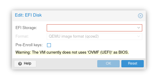
Add EFI disk, but do not check “pre-enroll keys”. This option would enroll keys and enable secure boot by default. Just add EFI disk without selecting this option and after starting VM you should be able to see your GPU in nvidia-smi.
Last time (somewhere around 2023) there was an option on Scaleway to install Proxmox 7 directly from appliance. There was also possiblity to use Debian 11 and install Proxmox atop of it. This time (2024/Nov) there is no direct install and installing on Debian gives me some unexpected errors which I do not want to overcome as it should work just like that.
But there is option to use Dell’s iDRAC interface for remote access.
In our lab we have 2 x HP z800 workstations. It is somehow ridiculous piece of hardware in terms of today standards. It’s got over 1 kW power supply, dual CPU motherboard and 12 memory slots. It is loud, draws loads of power and it’s got comparable gen 1 Intel CPUs as well as DDR3 – slow – memory. However it costs close to nothing and it is suitable for most small and mid applications.
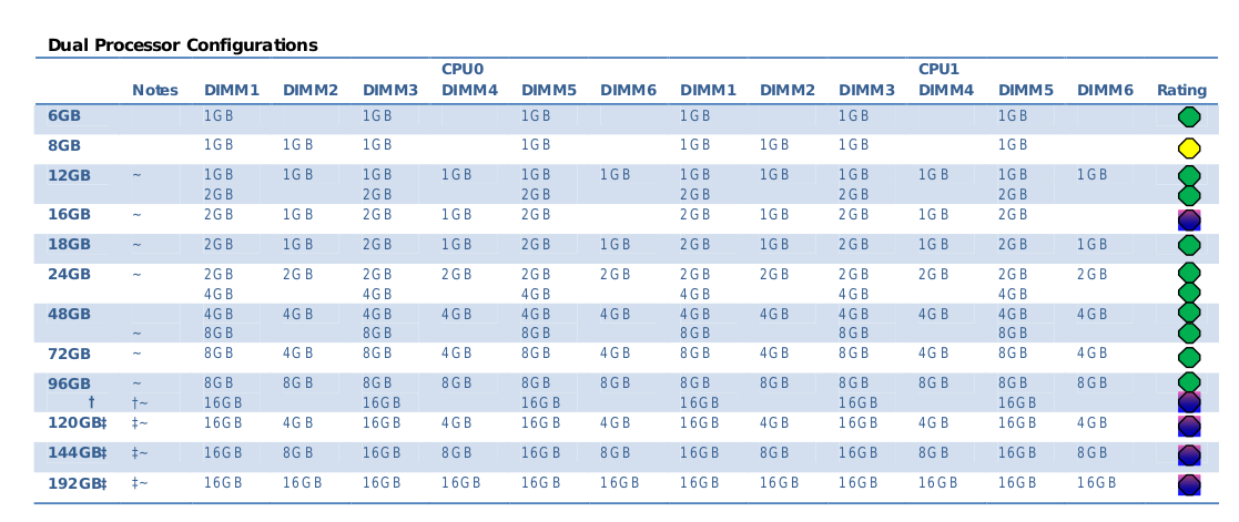
Official documentation says that the maximum memory capacity is 192GB of DDR3, which is 12 x 16 GB sticks working at 800 MHz. If we are interested in higher speeds, then we go to 96GB at 1067 MHz using 16GB sticks or 1333 MHz at all 8GB sticks. Currently (2025) DDR5 memory works up to 8800 MT/s, so it is roughly 10 times faster, however with higher latencies. Much higher clock speeds compensates higher latencies.
Even though having 384GB of DDR3 is a lot for regular computing like application servers, mail servers, file storage, surveillance etc. At our lab we are using this server for data mining which includes Docker containers as well as database servers (various types).
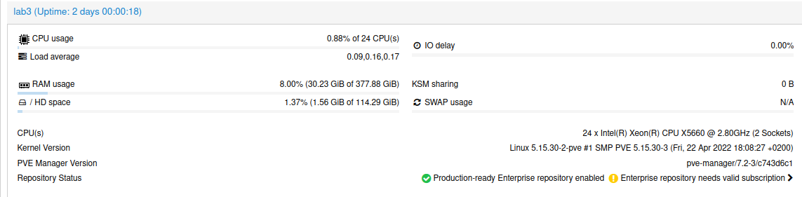
However, we can put more memory than 192GB. We put as twice as much. Actually, installing Intel Xeon x5660 we would be able to handle as much as 288GB per CPU giving 576 GB of RAM in total. But we have only 12 memory slots and maximum capacity of memory module is 32GB. If we would have 18 memory slots then we would be able to put 576 GB, but with 12 memory slots we are able to place “only” 384GB.
HP z800 motherboard and Xeon CPUs take both unbuffered and registered DIMMs but not at the same time. So be sure to buy only one type, which I think it should be either 8500R or 10600R. Is is not worth to buy faster DIMMS as they still will be working at 800MT/s.
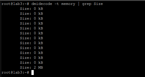
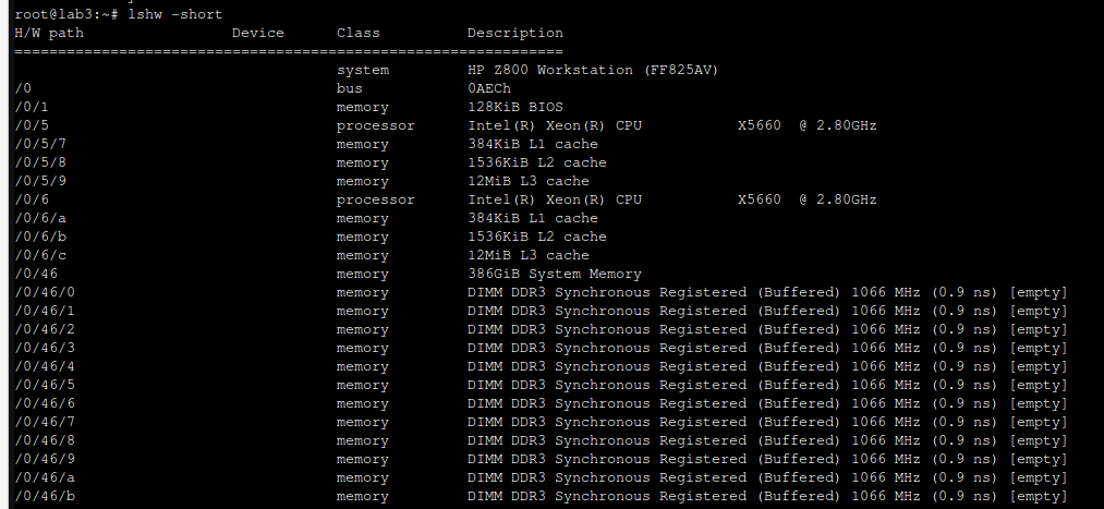
One important quirk regarding 32GB DDR3 memory sticks is that they are not recognized properly but dmidecode:
Same thing with lshw:
To access 12 x memory slots you need to remove double fan case. Moreover each memory module contains metal plate for heat dissipation. It can get really hot if put under heavy load.
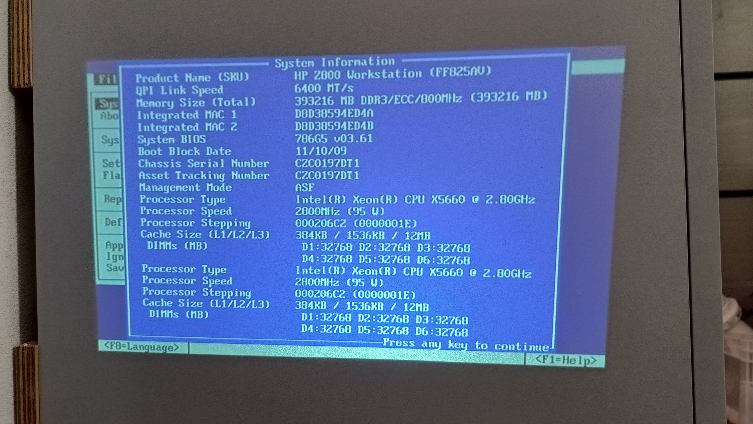
BIOS says that everything is fine. All DIMMS are recongnized. Each Xeon x5660 and x5690 has 3 memory channels so be sure to place same type/speed/latency memory module in 2 consecutive memory slots. As per documentation there is preffered way to populate memory sticks in case of placing less than maximum number of them, so be sure to either place 12x same sticks or follow documentation to have the most close confiugration.
To try installing 384GB of RAM I was inspired by https://www.youtube.com/watch?v=AoS0kX82vs4 – it worked out! Finall note. Regular market price of 32GB DDR3 sticks varies between 50 and 300 PLN (10 – 70 EUR). However I was able to find 24 sticks (as I we have 2 such servers) for as low as 7 EUR per stick. Few years back it would be cost of 1600 EUR, today it was 160 EUR.
I thought of adding another Proxmox node to the cluster. Instead of having PBS on separate physical box I wanted to have it virtualized, same as on any other environment I setup. So I installed fresh copy of the same Proxmox VE version and tried to join the cluster. And then this message came:
Connection error 500: RPCEnvironment init request failed: Unable to load access control list: Connection refused
And plenty other regarding hostname, SSH keys, quorum etc. Finally Proxmox UI went broke as I was unable to sign in. Restarting cluster services ended with some meaningless information. So I was a little bit worried about the situation. Of cource I got backup of all things running on that box, but it would be annoying to bring it back from backup.
Solution, or rather monkey-patch for this is to shutdown this new node. On any other working node (preferably on leader) execute:
umount -l /etc/pve
systemctl restart pve-cluster
This command unomunts and remounts FUSE filesystem and then restarts PVE cluster service. What was the root cause of this? Actually I do not know for sure, but I suspect either networking or filesystem issue causing some discrepancies on distributed configuration. I even added all node domains to local pfSense resolved to be sure that it is not DNS issue. Another options is that 2 out of 4 nodes have additional network interface with bridge. Different filesystems (ZFS vs XFS) might be a problem, but I do not think so anymore, as 2 nodes already got ZFS and adding them to cluster was without any problems in the past.
I decided not to restart any nodes or separate them as it might cause permanent obstruction. So it stays as a mistery, with monkey-patch to have it running once again.
If you have OpenHAB on Proxmox or any other virtualization and it sometimes fails to grab RTSP stream and create snapshots, then there is high chance that everything is fine with the camera and network and the problem is within your server hardware. I was investigating this matter a lot and came into this simple conclusion.
If camera does not have built snapshot URL coming from ONVIF (like on EasyCam WiFi with both ONVIF and Tuya) then your OpenHAB will try to make one from RTSP stream with ffmpeg. It starts ffmpeg process which will periodically (in my case every 2 seconds) grab frame and make JPEG out of it. However if you run your OpenHAB on some older hardware like I do (i3-4150 with 2c/4t) there is a chance that 100% utilization spikes on one vCore is too much for it… really. I noticed that with those CPU util spikes come also other connectivity issues and migrating OpenHAB to different server within the same cluster solved almost 100% the problem.
Instead of no image every minute or so now it misses snapshot every few hours. It might do this still because of WiFi signal strength and not because of lack of computational power on server side. There might be also case when camera is buy doing other things. Hikvision cameras notifies you with proper XML error code about this. Maybe there is also the case with EasyCam cameras. Who knows.
We took IP2Location version DB11 database. It holds few millions of IPv4 ranges which should unwrap onto over 2 billion addresses. Such number of entries is actually not a big deal for PostgreSQL RDBMS or Apache Cassandra distributed databases system. However there is an issue of ingestion speed. The question is how quick I can programmatically compute IP addresses for IP ranges and insert them in persistant storage.
PostgreSQL can hold easily around 10TB of data in single node. It can hold even more especially if divided into separate partitions/tables or use multiple tablespaces with separate drives. In case of Apache Cassandra it is said that it can hold also over 10 TB per node. So lets check it out!
Cassandra keyspace and table definition
We start with defining basic non-redundant keyspace. Non-redundand because we want to know about data structure layout first.
create table hosts_by_country_and_ip
(
  country varchar,
  ip varchar,
  region varchar,
  city varchar,
  lati varchar,
  longi varchar,
  izp varchar,
  timezone varchar,
  primary key ((country), ip)
);
With single partition key (country) and 6 Cassandra nodes (with default settings from Docker container) we get 8 – 9k inserts per second. It is way below of expected 20 – 40k inserts on modern hardware. However test setup is not run on modern hardware, it is actually run on HP Z800.
create table hosts_by_country_and_ip
(
  country varchar,
  ip varchar,
  region varchar,
  city varchar,
  lati varchar,
  longi varchar,
  izp varchar,
  timezone varchar,
  primary key ((country, region, city), ip)
);
Now with different table structure approach. Instead of single partition key, there are now 3 partition keys (country, region, city). Cassandra calculates partition key with token function which gives numeric result. By default each Cassandra node holds 16 tokens (token value ranges to be precise). Every insert calculates token value and coordinator places insert to appropriate node which holds the same token – holds data related to this token. With such a structure change, we get 16k inserts per second.
Why is that you may ask? It depends on data being inserted actually. So our ingestion Python program reads PostgreSQL IPv4 range and generates IP address list to insert into Cassandra. We did not put any kind of ORDER clause, so it may be or not be “random” data distribution. Effectively Cassandra write coordinator needs to solve too many conflicts/blockings because there are multiple runners inserting the same partition key data. If we spread out data we minimize conflicts solving computational time.
Cassandra node configuration
At first we tried to adjust table structure to increase writes performance. Next thing we can try on different hardware and with modified runtime parameters. So instead of HP Z800 (with SATA SSD drives) we run single Cassandra node on machine with single NVME drive. Created the same keyspace and the same table. With no change. Maybe there was a change, as single node outperformed 6 nodes, but we expect to have write thruput increased even more. No matter if this was 6, 12 or 24 Python ingestion instances running. We get up to 16k writes per second.
However additionally we set the following configuration values:
And increased MAX_HEAP_SIZE from 4GB to 8GB. We did not follow too much the documentation, but rather common-sense to increase write concurrency with arbirtary value. Run 24 Python ingestion instances and finally we got better results – 24k writes per second.
Measuring thruput
How to even measure write thruput easily? Cassandra do not offer any kind of analytics at that level. You need to manually created counters or use Spark to calculate count on token list. We choose the first approach. There are external counters which are updated with every Python runner. This way based on boolean logic, we can also achieve selecting data for concurrent processing.
Client-limited performance
Running only 12 Python ingestion instances gives over 18k writes per second. So there is link between server capabilities and running tasks inserting data. Increasing runners to 48 instances gives 28k writes per second. With 64 instances we got 29 – 30k writes per second. And I think is the max from the hardware and configuration at this time.
Reads vs Writes
There is one more thing to consider regarding performance. During intensive writes (e.g. 12 ingestion instances) CPU utilization oscillates around 200 – 300% (on 4 core, 8 thread CPU). However during intensive reads, with lets say, 32 parallel processes running, we can see CPU utilization between 400 and 700%. It is the level unseen during writes.
...

# Function processing single partition
def process_single_partition(r):
    cluster = Cluster(['0.0.0.0'])
    session = cluster.connect()
    session.execute("USE ip2location")
    stmt = session.prepare("SELECT ip as c FROM hosts_by_country_and_ip WHERE country=? AND region=? and city=?")
    res = session.execute(stmt, [r[0], r[1], r[2]])
    counter = 0
    for row in res:
        counter = counter + 1
    print(r, counter)

# Multiprocessing invocation
Parallel(n_jobs=32)(delayed(process_single_partition)(obj) for obj in records)
As both PostgreSQL and Cassandra sessions and not pickable by Parallel, we need to either use connection pool or simply create connection with each run. For this simple demo it is enough.
Due to distributed nature of Cassandra, we cannot simply run COUNT query. Even when using all the required partition columns. In this example those are country, region and city. Even with usage of all of them we will get timeouts running COUNT, and even if we do not run inserts during out counting procedure. Most probably, if we would enlongen particular timeout parameters we could get more results. Still using COUNT we will get some results, but it will not be reasonable way to actually count our records number. The proper one is to build structures holding data counters or use Cassandra diagnostics.
Notice: other possiblities to count are DSE Analytics, nodetool tablestats. DataStax Bulk Loader seems to be also interesting one.
More nodes and more drives
It is said that Cassandra scales easily just by adding additional nodes with additional drives preferably. Generally speaking it is true, but should also consider such parameters like server heap size, memory available and CPU performance. Even better performance will be achieved if storage backend will be constructed from multiple drives giving more IOPS. It is also important to remember that contrary to RDBMS, in Apacha Cassandra (Dynamo concept) we need to design structures by query usage and not by data organization.
Ever wondered what can be the highest load average on the unix-like system? Do we even know what this parameter tells about? It shows the average number of either actively running or waiting processes. It should be close to the number of logical processors present on the system, otherwise, in case it is greater than this, some things will need to wait in order to be executed.
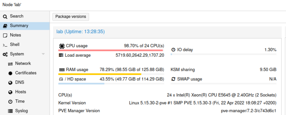
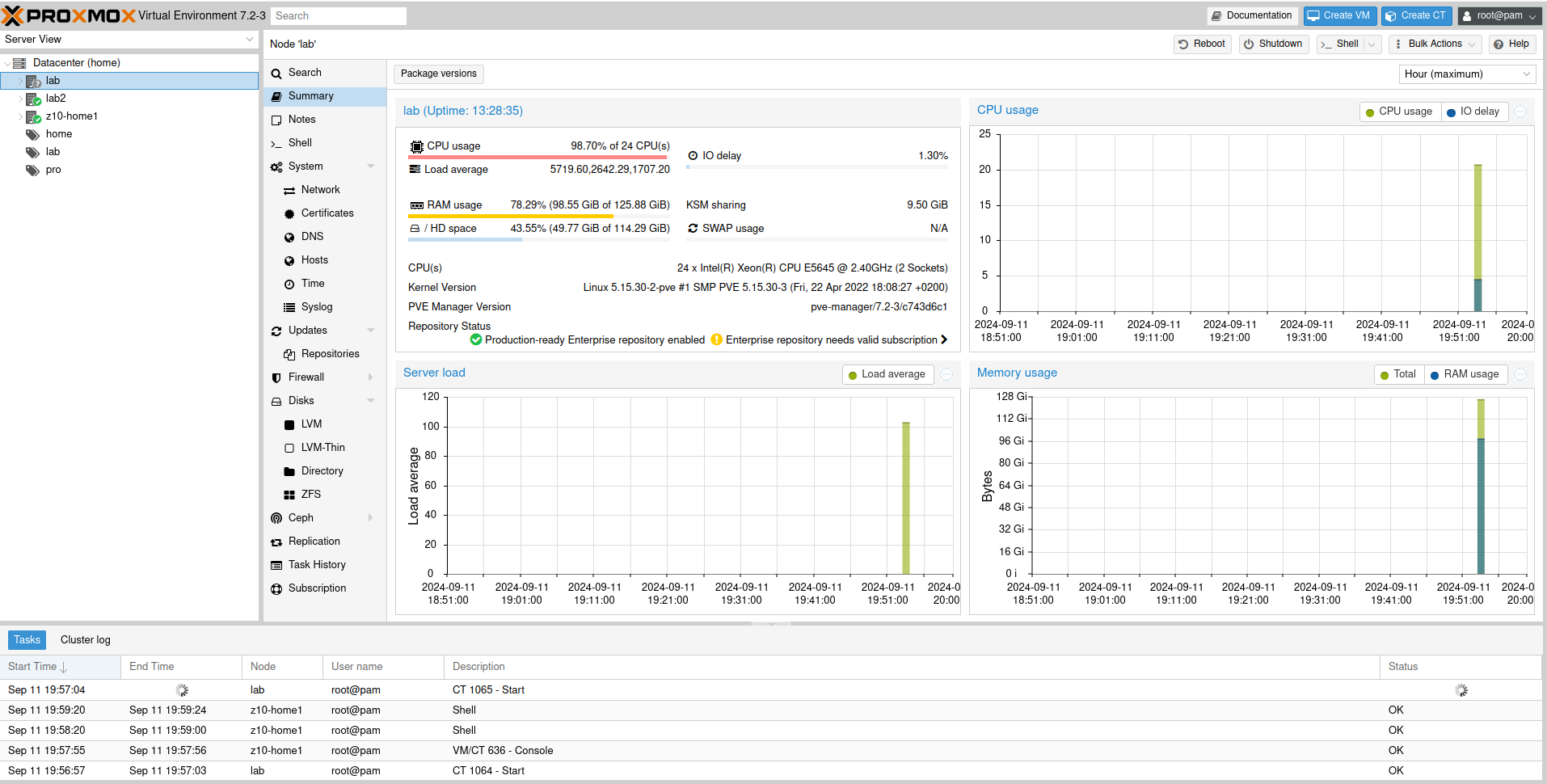
So I was testing 1000 LXC containers on the 2 x 6 core Xeon system (totalling as 24 logical processors) and leave it for a while. Once I got back I saw that there is something wrong with system responsiveness.
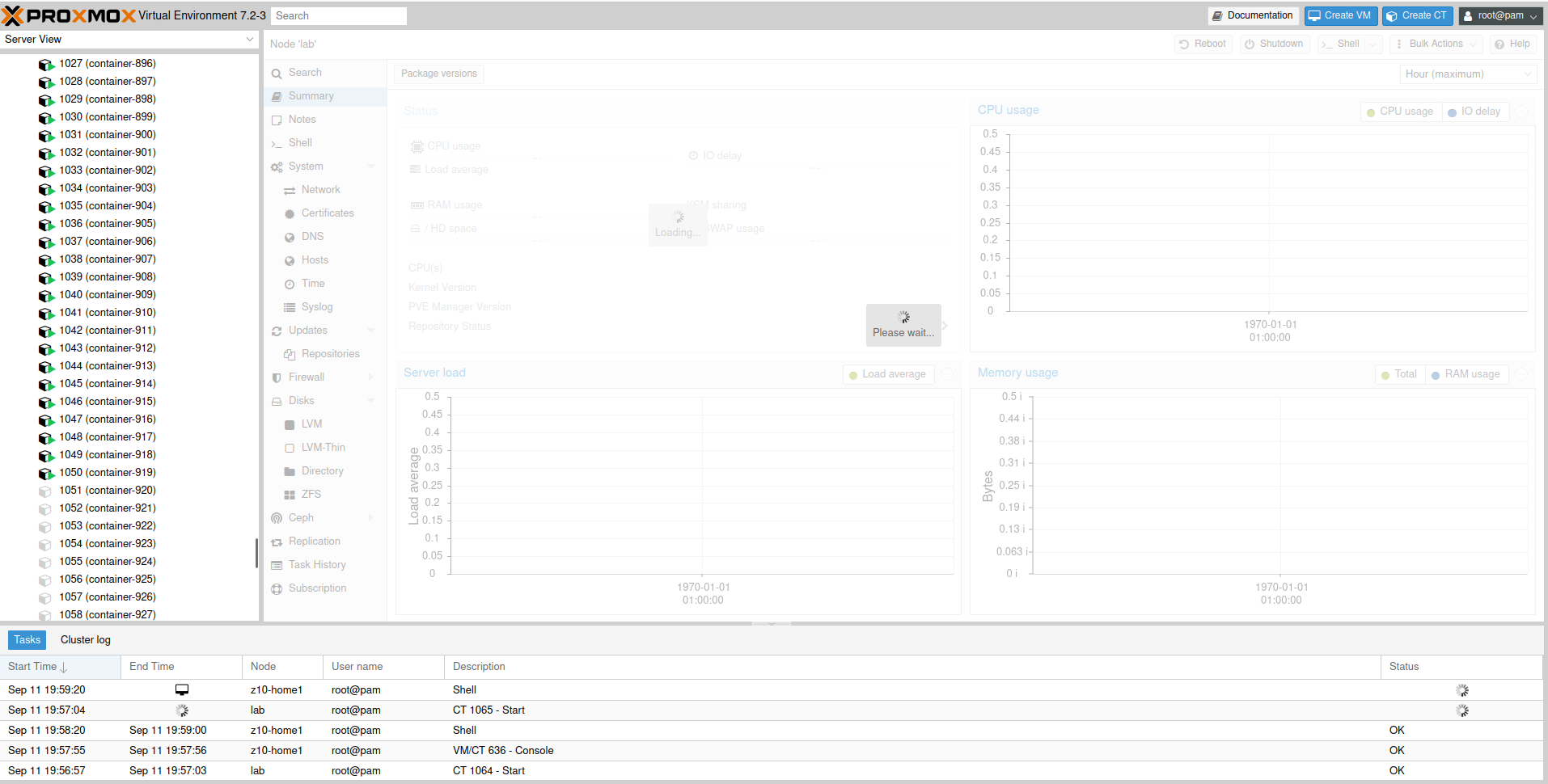
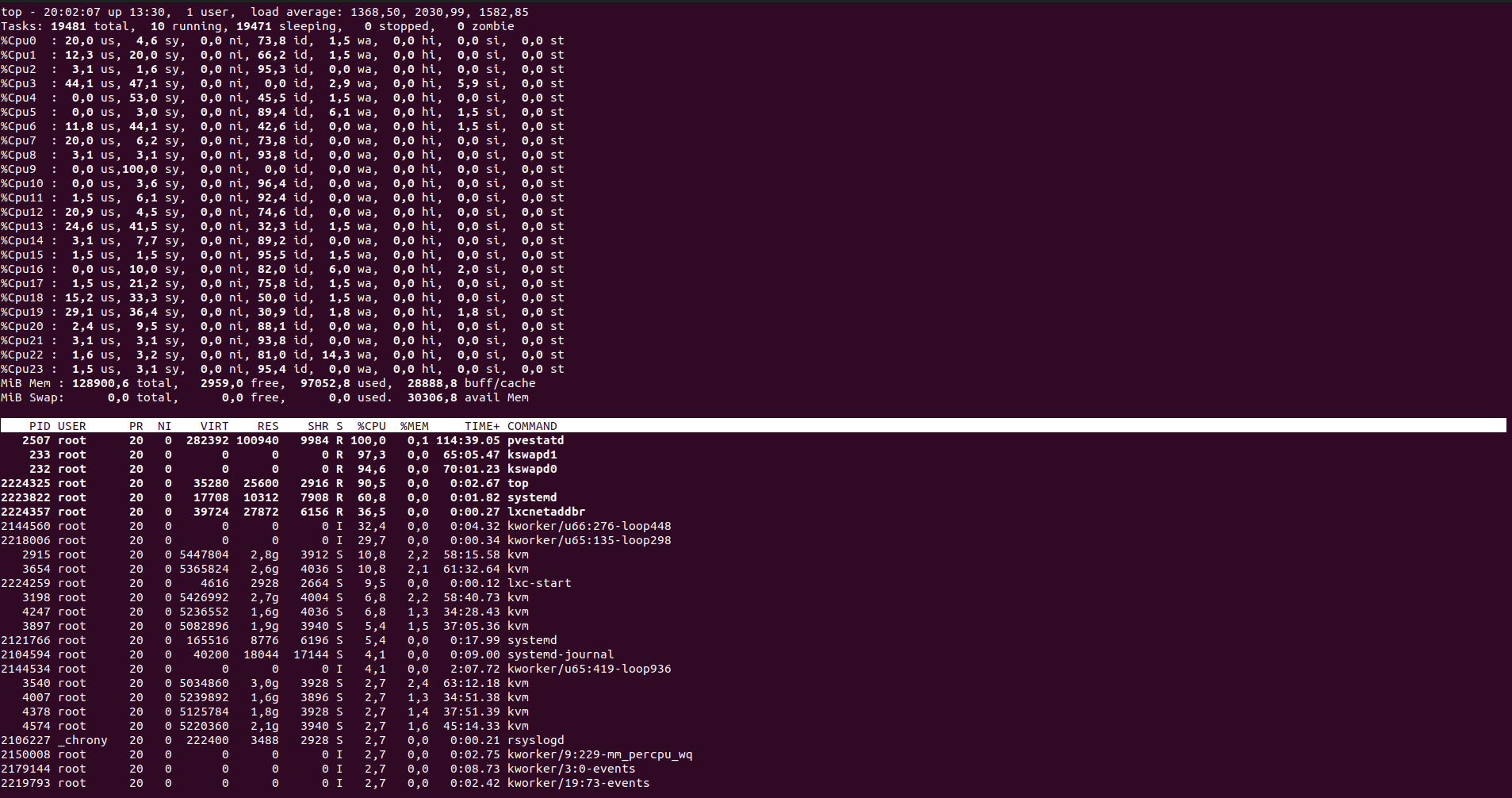
And my load average was 1min: 5719, 5 min: 2642, 15 min: 1707. I think that this the highest I have ever seen on systems under my supervision. What is interesing is that the system was not totally unresponsive, rather it was a little sluggish. Proxmox UI recorded load up to somewhere around 100 which should be a quite okey value. But then it sky-rocketed and Proxmox lost its ability to keep track of it.
I managed to login into the system and at that moment load average was already at 1368/2030/1582, which is way less than a few minutes before. I tried to cancel top command and reboot it, but even such trival operation was too much at that time.
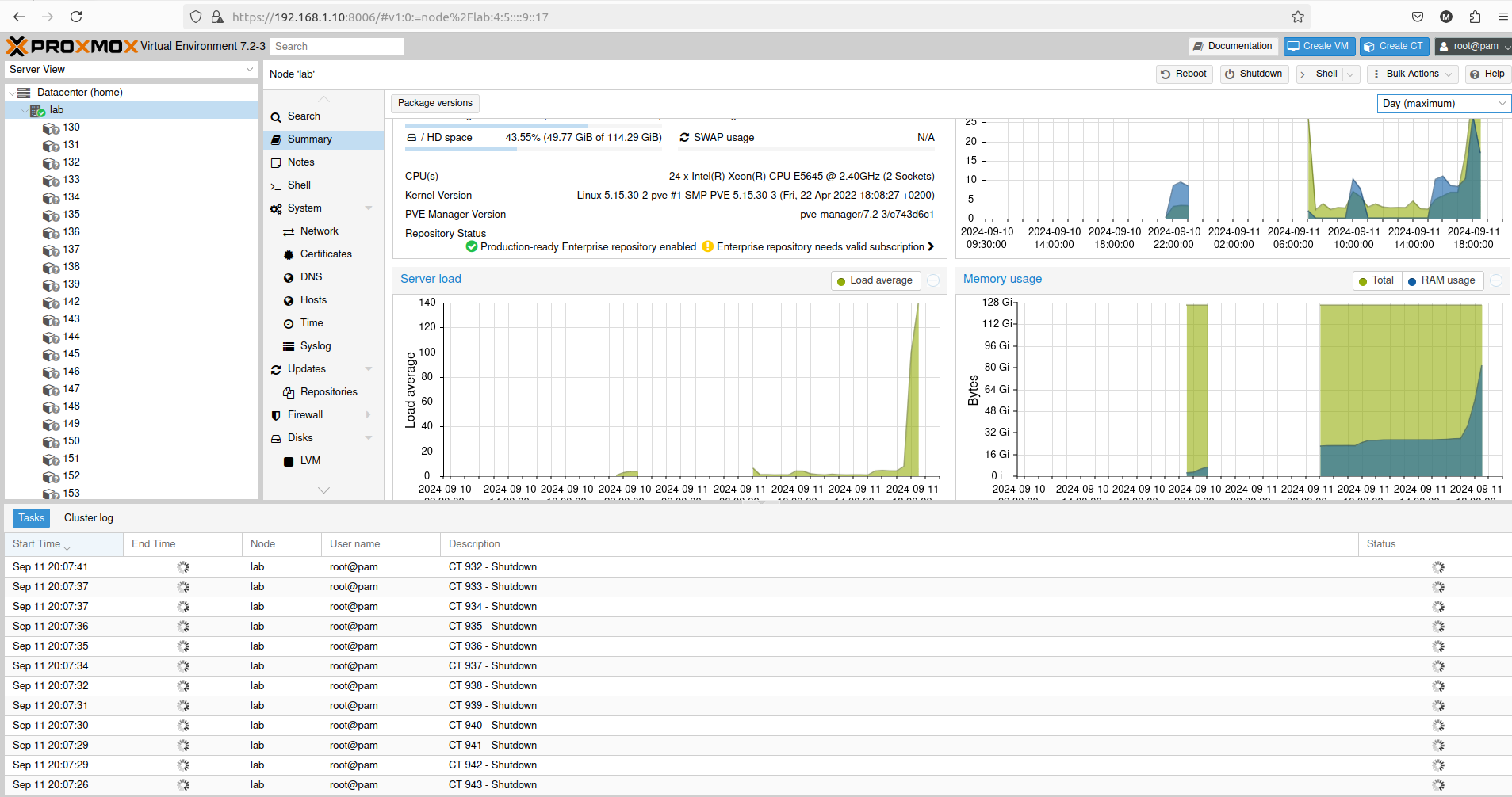
Once I managed to initiate system restart it started to shut down all those 1000 LXC containers present on the system. It took somwhere around 20 minutes to shut everything down and proceed with reboot.