IP2Location is a IP address databases where you can find the latest IP to location associations. The complete IPv4 range is 4 294 967 296 addresses which is 32 bit. IP2Location contains 4 291 944 710 addresses which is a little less. However as much as 608 487 295 addresses come with no location set. It is because of:
0.0.0.0/8 (local)
10.0.0.0/8 (class A)
100.64.0.0/10 (shared)
127.0.0.0/8 (host)
169.254.0.0/16 (link-local)
172.16.0.0/12 (class B)
192.0.0.0/24 (dual-stack)
192.0.2.0/24 (documentation etc)
192.88.99.0/24 (reserved, IPv6 to IPV4)
192.168.0.0/16 (class C)
198.18.0.0/15 (benchmarking)
198.51.100.0/24 (documentation etc)
203.0.113.0/24 (documentation etc)
224.0.0.0/4 (multicast, class D)
233.252.0.0/24 (documentation etc)
240.0.0/4 (reserved, class E)
255.255.255.255/32 (broadcast)
Above should not have location set as those are special IPv4 ranges. So valid commercial (and non-commercial also) use IPv4 addresses count should be somewhere near value of 3 683 457 415, which is all addresses minus addresses without location. DARPA developed IPv4 started in 1981 and has been exhausted in 2011.
How does this apply to Cassandra databases?
Complete 3.6B addresses weights around 40GB of data in single Apache Cassandra 5.0 node. Using commodity hardware with Intel i5 10200H and Western Digital SN530 NVME drive we can get up to 29k inserts per second. Doing the math the complete ingestion should finish within 35 hours. However if we would put multiple Cassandra nodes to split writes it most probably be much faster. Lets say we would run at 100k/s so ingestion time would be 10 hours. With 1M/s this would run for only 1 hour.
We took IP2Location version DB11 database. It holds few millions of IPv4 ranges which should unwrap onto over 2 billion addresses. Such number of entries is actually not a big deal for PostgreSQL RDBMS or Apache Cassandra distributed databases system. However there is an issue of ingestion speed. The question is how quick I can programmatically compute IP addresses for IP ranges and insert them in persistant storage.
PostgreSQL can hold easily around 10TB of data in single node. It can hold even more especially if divided into separate partitions/tables or use multiple tablespaces with separate drives. In case of Apache Cassandra it is said that it can hold also over 10 TB per node. So lets check it out!
Cassandra keyspace and table definition
We start with defining basic non-redundant keyspace. Non-redundand because we want to know about data structure layout first.
create table hosts_by_country_and_ip
(
  country varchar,
  ip varchar,
  region varchar,
  city varchar,
  lati varchar,
  longi varchar,
  izp varchar,
  timezone varchar,
  primary key ((country), ip)
);
With single partition key (country) and 6 Cassandra nodes (with default settings from Docker container) we get 8 – 9k inserts per second. It is way below of expected 20 – 40k inserts on modern hardware. However test setup is not run on modern hardware, it is actually run on HP Z800.
create table hosts_by_country_and_ip
(
  country varchar,
  ip varchar,
  region varchar,
  city varchar,
  lati varchar,
  longi varchar,
  izp varchar,
  timezone varchar,
  primary key ((country, region, city), ip)
);
Now with different table structure approach. Instead of single partition key, there are now 3 partition keys (country, region, city). Cassandra calculates partition key with token function which gives numeric result. By default each Cassandra node holds 16 tokens (token value ranges to be precise). Every insert calculates token value and coordinator places insert to appropriate node which holds the same token – holds data related to this token. With such a structure change, we get 16k inserts per second.
Why is that you may ask? It depends on data being inserted actually. So our ingestion Python program reads PostgreSQL IPv4 range and generates IP address list to insert into Cassandra. We did not put any kind of ORDER clause, so it may be or not be “random” data distribution. Effectively Cassandra write coordinator needs to solve too many conflicts/blockings because there are multiple runners inserting the same partition key data. If we spread out data we minimize conflicts solving computational time.
Cassandra node configuration
At first we tried to adjust table structure to increase writes performance. Next thing we can try on different hardware and with modified runtime parameters. So instead of HP Z800 (with SATA SSD drives) we run single Cassandra node on machine with single NVME drive. Created the same keyspace and the same table. With no change. Maybe there was a change, as single node outperformed 6 nodes, but we expect to have write thruput increased even more. No matter if this was 6, 12 or 24 Python ingestion instances running. We get up to 16k writes per second.
However additionally we set the following configuration values:
And increased MAX_HEAP_SIZE from 4GB to 8GB. We did not follow too much the documentation, but rather common-sense to increase write concurrency with arbirtary value. Run 24 Python ingestion instances and finally we got better results – 24k writes per second.
Measuring thruput
How to even measure write thruput easily? Cassandra do not offer any kind of analytics at that level. You need to manually created counters or use Spark to calculate count on token list. We choose the first approach. There are external counters which are updated with every Python runner. This way based on boolean logic, we can also achieve selecting data for concurrent processing.
Client-limited performance
Running only 12 Python ingestion instances gives over 18k writes per second. So there is link between server capabilities and running tasks inserting data. Increasing runners to 48 instances gives 28k writes per second. With 64 instances we got 29 – 30k writes per second. And I think is the max from the hardware and configuration at this time.
Reads vs Writes
There is one more thing to consider regarding performance. During intensive writes (e.g. 12 ingestion instances) CPU utilization oscillates around 200 – 300% (on 4 core, 8 thread CPU). However during intensive reads, with lets say, 32 parallel processes running, we can see CPU utilization between 400 and 700%. It is the level unseen during writes.
...

# Function processing single partition
def process_single_partition(r):
    cluster = Cluster(['0.0.0.0'])
    session = cluster.connect()
    session.execute("USE ip2location")
    stmt = session.prepare("SELECT ip as c FROM hosts_by_country_and_ip WHERE country=? AND region=? and city=?")
    res = session.execute(stmt, [r[0], r[1], r[2]])
    counter = 0
    for row in res:
        counter = counter + 1
    print(r, counter)

# Multiprocessing invocation
Parallel(n_jobs=32)(delayed(process_single_partition)(obj) for obj in records)
As both PostgreSQL and Cassandra sessions and not pickable by Parallel, we need to either use connection pool or simply create connection with each run. For this simple demo it is enough.
Due to distributed nature of Cassandra, we cannot simply run COUNT query. Even when using all the required partition columns. In this example those are country, region and city. Even with usage of all of them we will get timeouts running COUNT, and even if we do not run inserts during out counting procedure. Most probably, if we would enlongen particular timeout parameters we could get more results. Still using COUNT we will get some results, but it will not be reasonable way to actually count our records number. The proper one is to build structures holding data counters or use Cassandra diagnostics.
Notice: other possiblities to count are DSE Analytics, nodetool tablestats. DataStax Bulk Loader seems to be also interesting one.
More nodes and more drives
It is said that Cassandra scales easily just by adding additional nodes with additional drives preferably. Generally speaking it is true, but should also consider such parameters like server heap size, memory available and CPU performance. Even better performance will be achieved if storage backend will be constructed from multiple drives giving more IOPS. It is also important to remember that contrary to RDBMS, in Apacha Cassandra (Dynamo concept) we need to design structures by query usage and not by data organization.
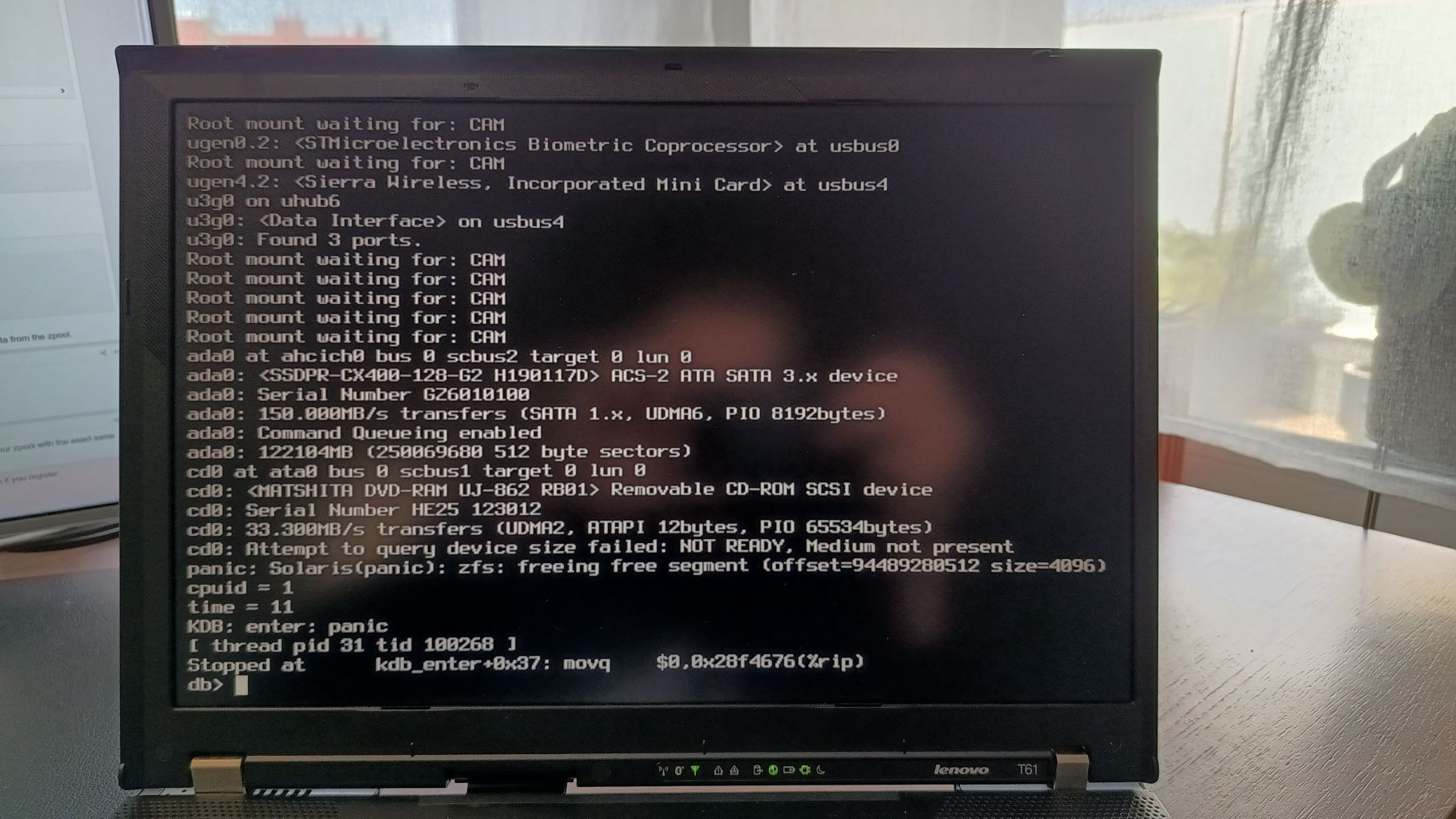
Recently my pfSense running on the same hardware for almost 3 years, died. I tried rebooting it and removing RAM, cards etc, with no luck. So decided to bring it back from configuration backup onto new drive. But after few days I stared investigating this matter and I got some temporary solution to start it back.
Here is how kernel panic looks like. It says: “Attempt to query device size failed” and “zfs: freeing free segment”. The latter is the cause of the problem with system starting up.
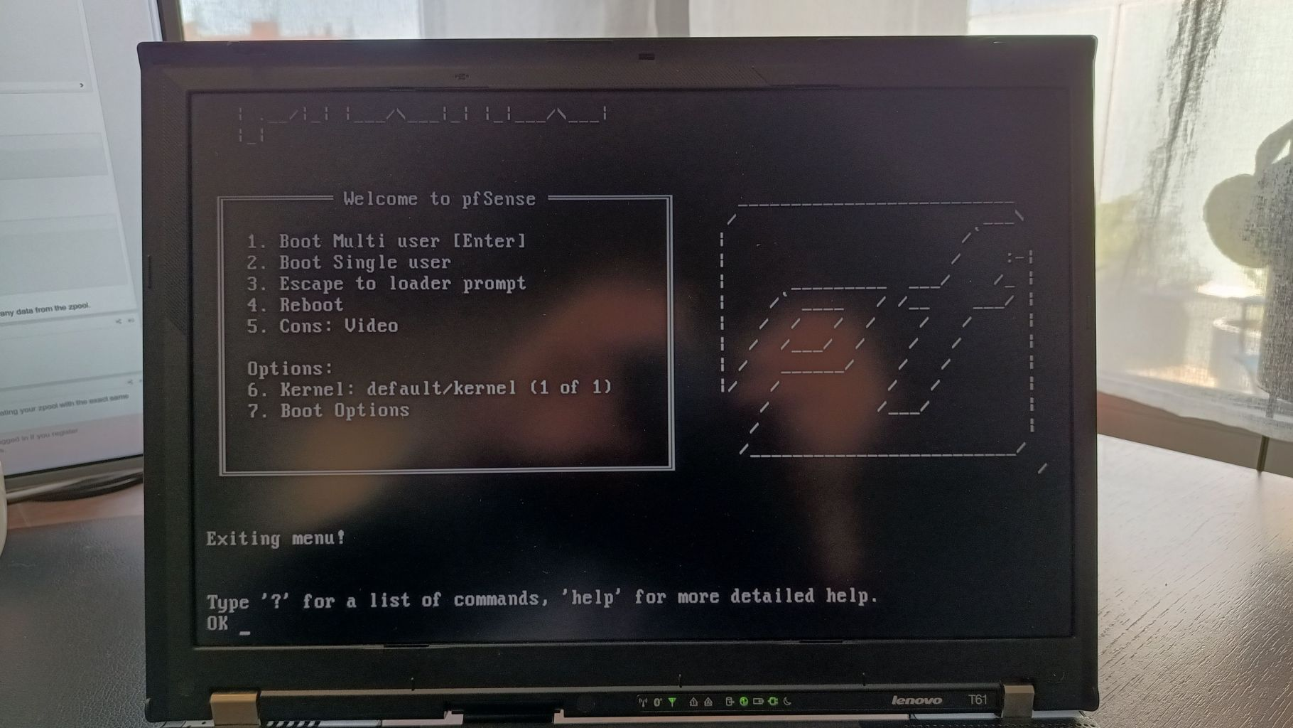
First, select “3” to escape to loader prompt:
Then set:
vfs.zfs.recover=1
vfs.zfs.debug=1
boot
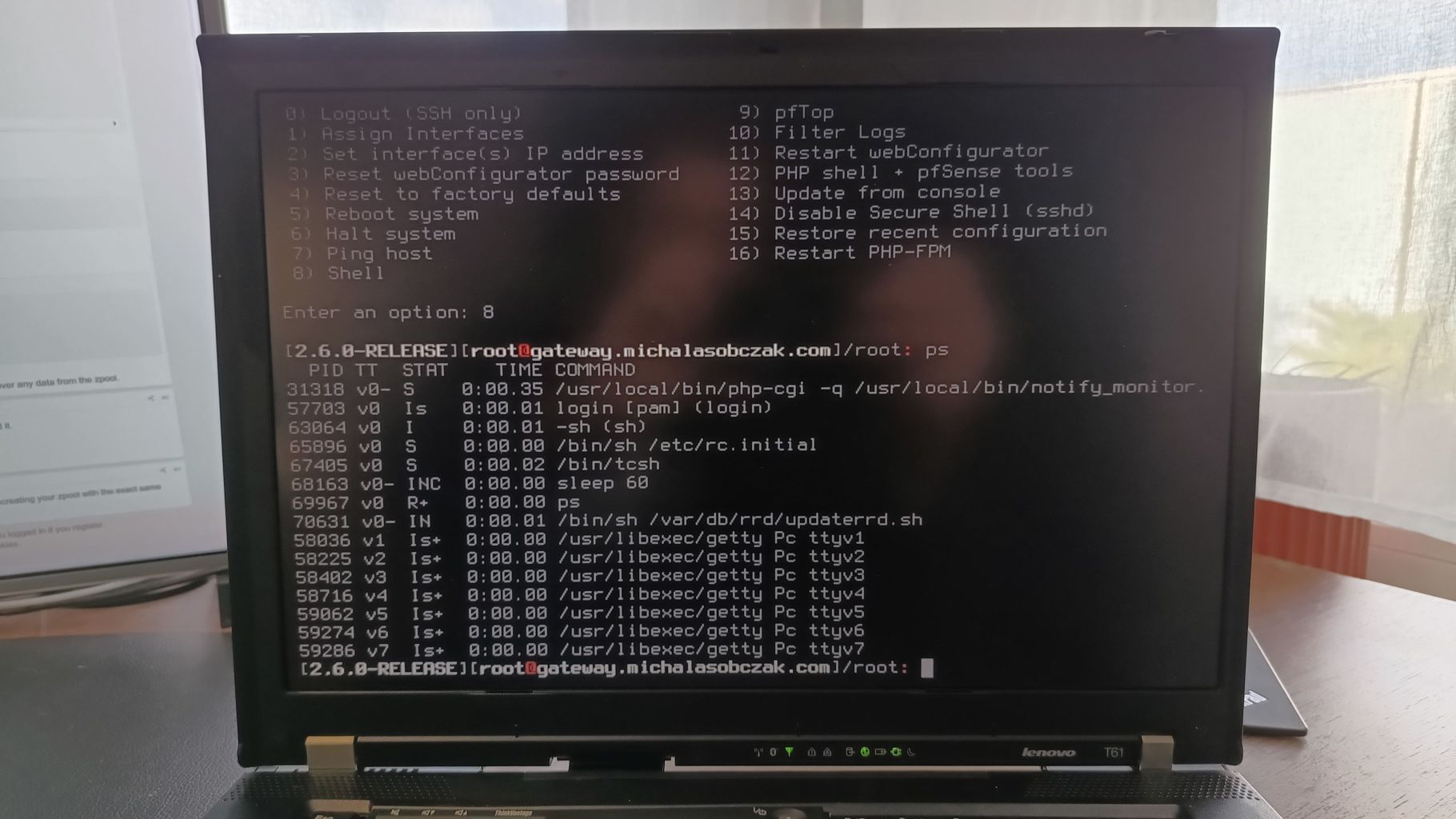
And you are in. However, now you need to verify if data is present, not corrupted and finally fix ZFS pool/sets as it is only a temporary fix and most probably still requires some manual work to be done.
Distributed, partitioned, multi-master, increment horizontal scale-out NoSQL data manegement system for global mission-critical use cases handling petabyte sized datasets
“Reliability at massive scale is one of the biggest challenges we face at Amazon“
source: “Dynamo: amazon’s highly available key-value store”
In 2004 there have been performance issues in Amazon e-commerce handling due to high traffic. By 2007 the concept of Dynamo has been materialized as Amazon S3. Then in 2008 Facebook with co-authors of Amazon Dynamo developed its own distributed NoSQL system, Cassandra. In 2009 Cassandra became Apache’s project. However, Amazon’s DynamoDB came in 2012, it also uses Dynamo concept, however it is fully proprietary solution.
So we have Dynamo concept, we have Amazon and Facebook and finally Apache Cassandra project. Without diving deep into the details of who was the first and who borrowed what… Cassandra is on the market for 16 years already (as of 2024).
Characteristics
Cassandra is meant to be run in multi-node environment and it is especially useful when running in dispersed networks. It is master-less which means that there is no single point of failure, of course only in case of proper keyspace/database and table designs especially in terms of replication factor. Having replication factor greater than 1, means that we introduce redundancy into our data layout which leads us towards resilience of a Cassandra cluster. Cassandra being distributed-capable still is visible as a single entity from user perspective.
The key concept which provides almost endless scaling capabilities is that Cassandra is distributed and uses data partitions. Comparing to RDBMS (like PostgreSQL) you need no additional configuration in order to run partitions and shards as it is built into Cassandra engine. Data in Cassandra are placed on particular nodes taking into account the partition key. If you need more storage or more computational power, you just add additional nodes to the cluster.
“Each node owns a particular set of tokens, and Cassandra distributes data based on the ranges of these tokens across the cluster.”
Data is spread across cluster based on partition key which is a hash-function value of data key which then maps to nodes which hold this particular tokens. Any node act as a coordinator looking for target node and gossiping with other nodes about cluster structure. There are of course many challanges, for instance when you defined replication factor > 1 and experience some networking issues. Transactions may or may not be successful depending on configuration, how many of nodes responded to transaction and confirmed it.
Concerning data placement strategy: for non-production or simple production setups you can use SimpleStrategy, however for bigger production setups it is recommended to use NetworkTopologyStrategy which take into consideration DC and Rack definitions.
“Data modeling that considers the querying patterns and assigns primary keys based on the queries will have the lowest latency in fetching data”
“Sorted Strings Table (SSTable) is a persistent file format used by ScyllaDB, Apache Cassandra, and other NoSQL databases to take the in-memory data stored in memtables, order it for fast access, and store it on disk in a persistent, ordered, immutable set of files. Immutable means SSTables are never modified. They are later merged into new SSTables or deleted as data is updated.”
source: www.scylladb.com/glossary/sstable/
Cassandra QL quirks
Keep mind that…
“The append and prepend operations are not idempotent by nature”
“lists have limitations and specific performance considerations that you should take into account before using them”
Currently, aliases aren’t recognized in the WHERE or ORDER BY clauses in the statement. You must use the orignal column name instead.
The primary key uniquely identifies a row in the table, as described above. A consequence of this uniqueness is that if another row is inserted using the same primary key, then an UPSERT occurs and an existing row with the same primary key is replaced. Columns that are not part of the primary key cannot define uniqueness.
…but as Cassandra allows the client to provide any timestamp on any table, it is theoretically possible to use another convention. Please be aware that if you do so, dropping a column will not correctly execute.
What I find interesting
I think that worth noticing is speculative_retry feature which defines when query coordinator could query another node for data in case of slow response or unavailability of some node.
Worth trying out is Vector Search feature:
Vector Search is a new feature added to Cassandra 5.0. It is a powerful technique for finding relevant content within large datasets and is particularly useful for AI applications.
I find in documentation that it is not recommended to run Cassandra on NFS/SAN as the whole Cassandra distrubuted concept relies on separated nodes. However it also told that Cassandra will better perform in RAID0 or JBOD (Just Bunch Of Disk) rather than on RAID1 or RAID5. Well… that is obvious that things run better without additional overhead, and I think that it should be stated that this suggestion is valid only if we aim for maximum performance sacrificing a little bit of security.
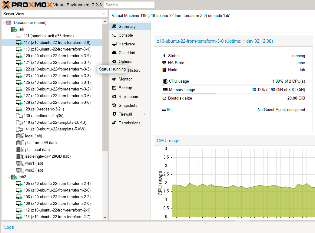
Installation in Docker/Portainer/Proxmox
In order to start with Cassandra we can use Proxmo virtual environment and Docker Swarm with Portainer on top of it. However, there are some certain issues with running it in Swarm mode. Long story short, Swarm adds additional ingress layer which adds additional IP addresses to the container. It somehow confuses Cassandra. I belive that there is some solution for this, however I found few bug reports in this matter without clear conclusion.
So, we can stay with Swarm mode, but deploy Cassandra as regular container, not a service. Yes, we can run regular containers without putting them into services while running in Swarm mode.
I will use previously prepared Docker Swarm cluster.
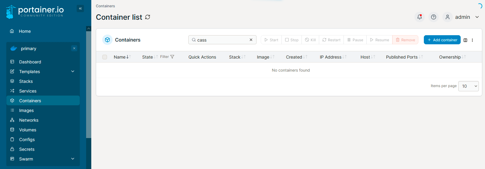
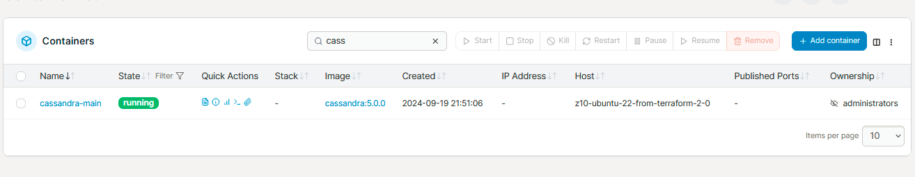
For this deployment I will go for Docker image cassandra:5.0.0:
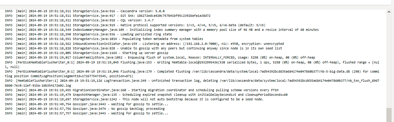
And here it starts:
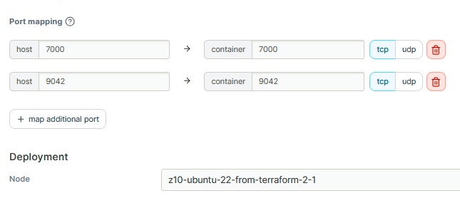
Every Cassandra node should open port 7000 for inter-node communication. Port 9042 is for query handling.
We need to point exact Docker Swarm node on which we would like to place our Cassandra node. Then in environments section define CASSANDRA_BROADCAST_ADDRESS and CASSANDRA_SEEDS. It is important to pass seed nodes cross cluster, so in case of outage everything left in the cluster should remain operational.
Monitoring nodes
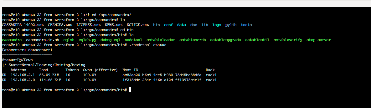
Every node container contains nodetool utility which helps identifing status of our Cassandra cluster. We can query for general status (status command), detaled info (info command), initialite compatcion (compact command) and many many more.
cd /opt/cassandra/bin
./nodetool status
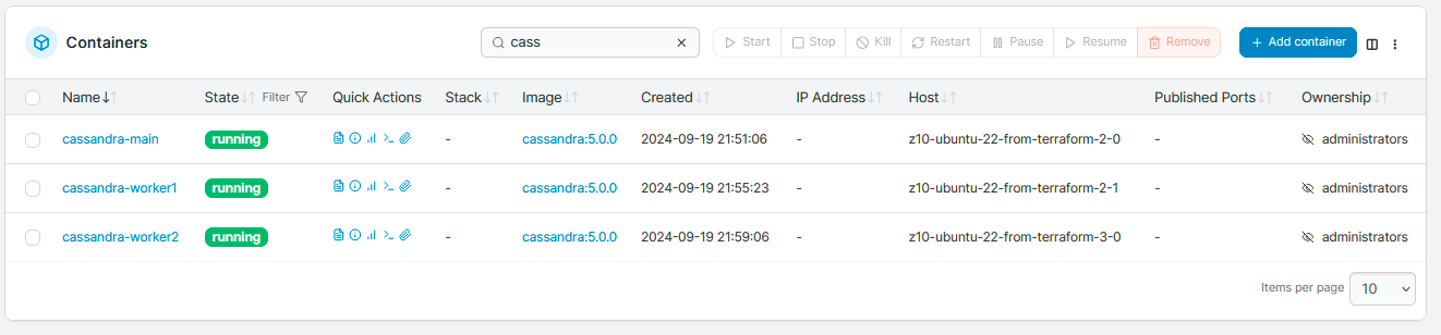
For this demo I decide to go for simple strategy cluster with one main node for seeding and two workers.
Data analysis with Redash
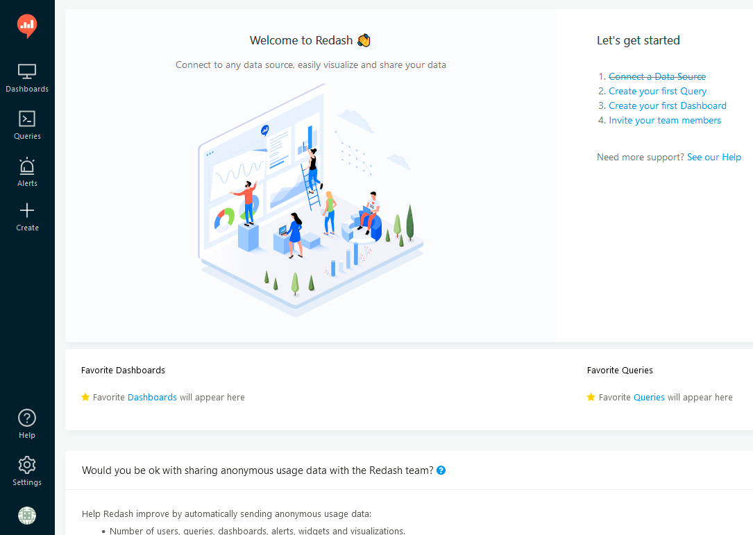
To query Cassandra you can use either CQLSH (present on every Cassandra node, /opt/cassandra/bin) or install Redash. It is a complete data browsers and visualizer with ability to connect to all major RDBMS and to Cassandra also. To install redash download https://github.com/getredash/setup repository and follow instructions.
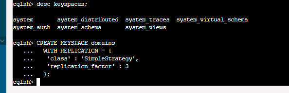
To start playing with CQL (Cassandra Query Language) we need to define keyspace (using CQLSH), which is some sort of database. We define it as SimpleStrategy with 3 copies. So all of our data will be spread on all cluster nodes. This way we will be resilient of hardware or network failure. For more complex scenarios use NetworkTopologyStrategy with defined DC and Rack parametrs.
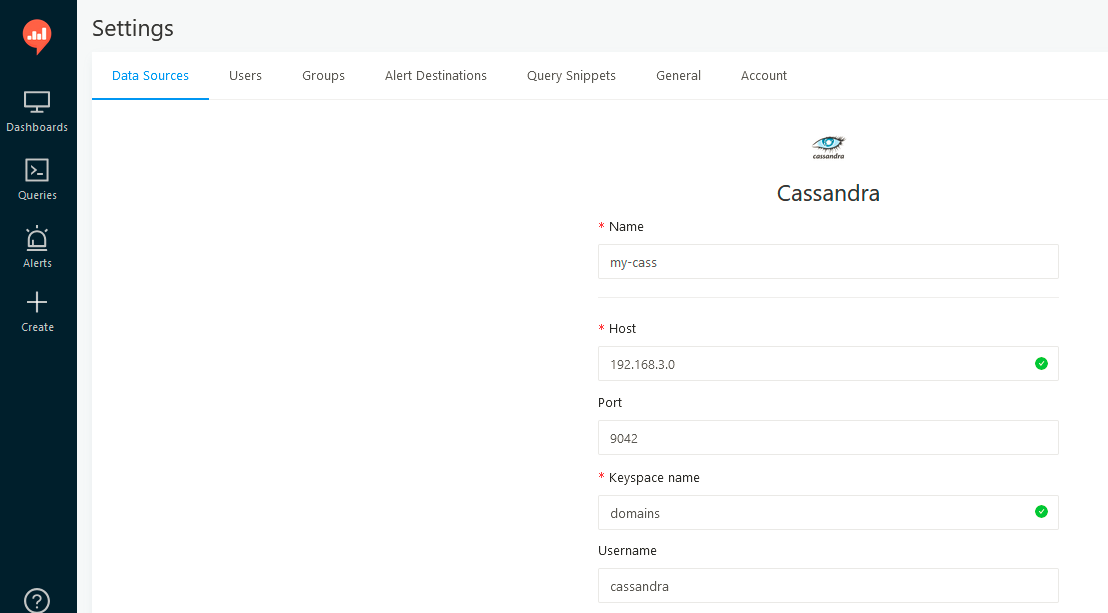
Now, once we created keyspace, we can go to Redash and define Data Source.
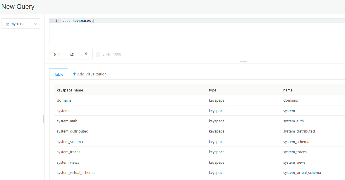
Then, start new query and play around.
CQL DDL
We already created keyspace/database, and it time to create table with single-column primary key.
create table mylist
(
  myid int primary key,
  mytext text
)
In return in Redash you will get:
Error running query: 'NoneType' object is not iterable
which means that Redash expects to receive an iterable object and instead of got nothing, because creating table or keyspaces returns nothing.
CQL DML
Cassandra restricts user as it limits possiblities to query for data only if clause matches primary key columns.
insert into mylist (myid, mytext) values (1, 'test 1');
insert into mylist (myid, mytext) values (2, 'test 2');

select * from mylist where myid = 1;
select * from mylist where myid in (1,2);
insert into myotherlist (myid, myotherid, mylastid) values (1, 1, 1);
insert into myotherlist (myid, myotherid, mylastid) values (2, 2, 2);
insert into myotherlist (myid, myotherid, mylastid) values (3, 3, 3);
insert into myotherlist (myid, myotherid, mylastid) values (4, 4, 4);
And then try various combinations of where clause. The following will return error “column cannot be restricted as preceding column is not restricted”. It means that it does not have individual indices which could help locate those different column values. Instead it seems that it have some kind of tree-like index structure (Log Structured Merge Tree to be specific) which can be traversed only by using all consecutive and adjacent primary key ingredients:
select * from myotherlist where mylastid = 1;
But this one will work:
select * from myotherlist where myid = 1;
select * from myotherlist where myid = 2 and myotherid = 2;
select * from myotherlist where myid = 3 and myotherid = 3 and mylastid = 3;
As primary key must be unique then you cannot insert same values in all columns which already exist in a table. Moreover, you cannot skip any or required clustering keys (myotherid and mylastid).
Same applies with partition key (myid):
Design principals
Contrary to RDBMS, Cassandra’s design principals are focused more on denomalization than normalization. You need to design your data model by the way you will be using it, intead of just describing the schema.
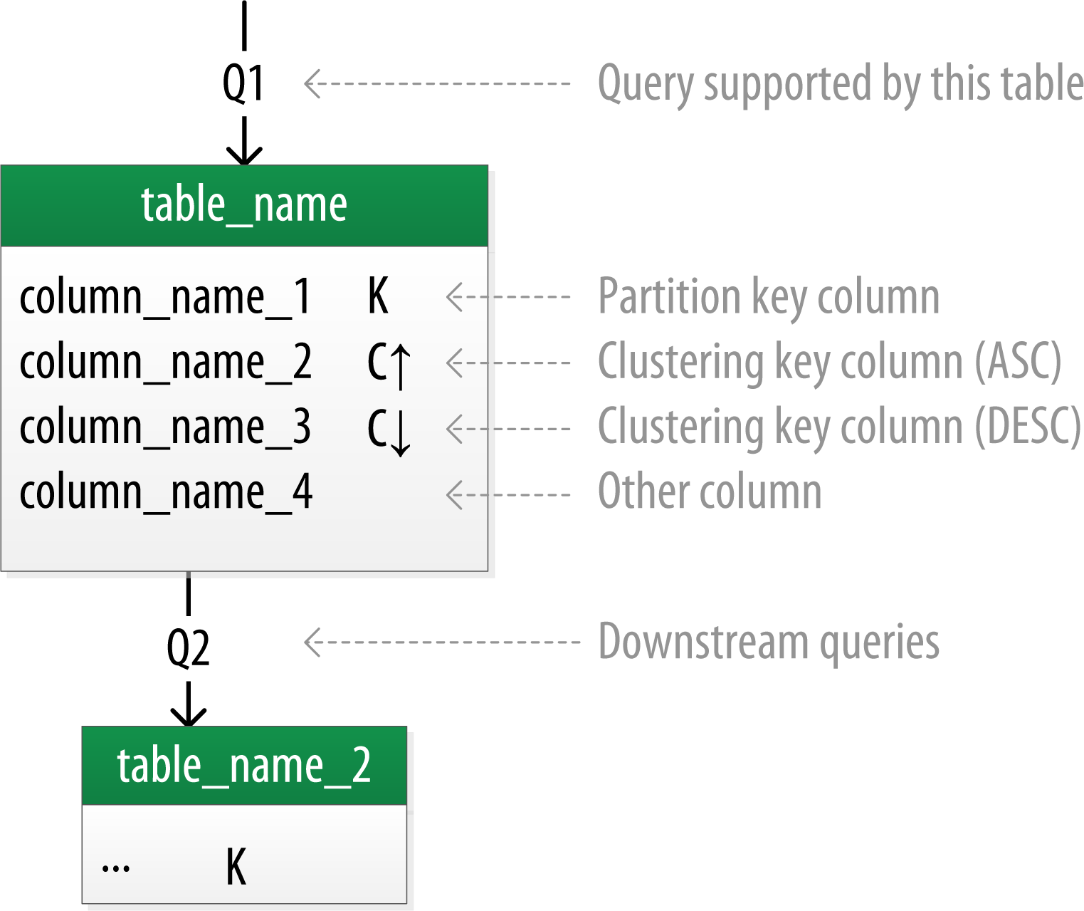
By contrast, in Cassandra you don’t start with the data model; you start with the query model
The sort order available on queries is fixed, and is determined entirely by the selection of clustering columns you supply in the CREATE TABLE command
In relational database design, you are often taught the importance of normalization. This is not an advantage when working with Cassandra because it performs best when the data model is denormalized.
A key goal that you will see as you begin creating data models in Cassandra is to minimize the number of partitions that must be searched in order to satisfy a given query. Because the partition is a unit of storage that does not get divided across nodes, a query that searches a single partition will typically yield the best performance.
Application example & flushing commitlog
So, previously I defined table called myotherlist with three integer colums contained in primary key. Let’s use Python to insert some data. First install the driver:
pip3 install cassandra-driver
Then define the program. We are going to use prepared statements as they save CPU cycles.
import cassandra
print(cassandra.__version__)

from cassandra.cluster import Cluster

cluster = Cluster(['192.168.2.0', '192.168.2.1', '192.168.3.0'])
session = cluster.connect()

ret = session.execute("USE domains")

rangeofx = range(100)
rangeofy = range(100)
rangeofz = range(100)

stmt = session.prepare("INSERT INTO myotherlist (myid, myotherid, mylastid) values (?, ?, ?)");

for x in rangeofx:
    for y in rangeofy:
        for z in rangeofz:
            print(x, y, z)
            session.execute(stmt, [x, y, z])
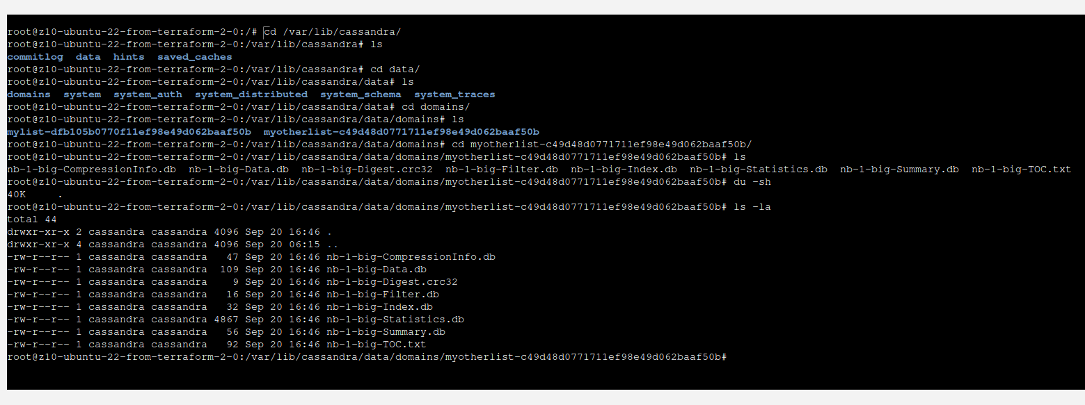
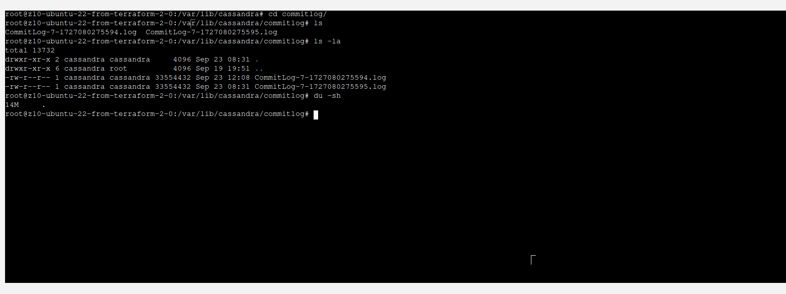
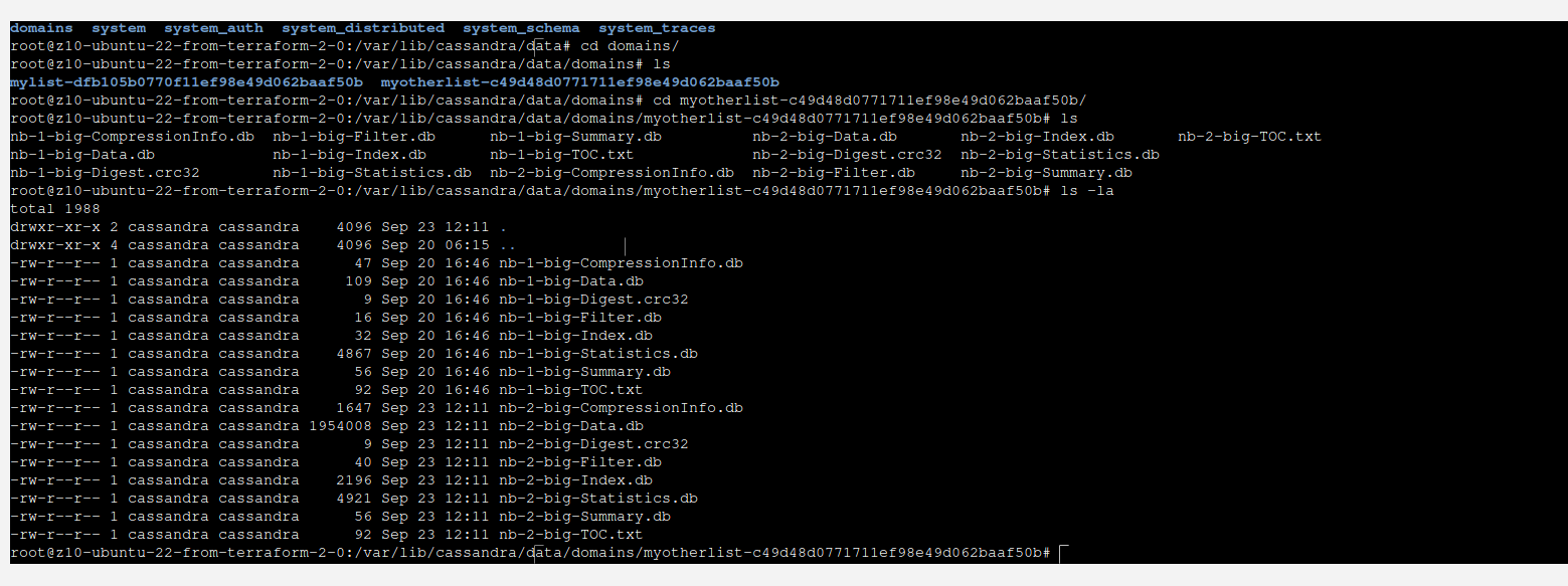
It is quite interesting that those data will not be present in data file instantly. Instead they will appear in commitlog, lets take a look:
You can see that there is not much happening here. However, when we take a look at commitlog, we can see that most probably there is our data located.
In order to write our data into SSTable files, you run ./nodetool flush. This will move memory and commitlog into data file.
Have you ever wondered how many tables can we create and use in PostgreSQL database server? Shall we call them partitions or shards? Why not to use built-in “automatic” partitioning?
Partitions or shards?
Lets first define the difference between partitions and shards. Partitions are placed on the same server, but shards can be spread across various machines. We can use inheritance or more recent “automatic” partitioning. However both of these solutions lead to tight join with PostgreSQL RDBMS, which in some situations we would like to avoid. Imagine a perspective of migrating our schemas to different RDBMS like Microsoft SQL Server. Not using any vendor-specific syntax and configuration would be beneficial.
Vendor agnostic partitions
So instead, we can just try to create partition-like tables manually:
Then, after installing PostgreSQL and creating new database:
for i in `seq 1 10000`;
do
  echo $i;
  psql -c "create table demo_$i (id int, val int);" partitions;
done
This way we created 10 000 tables with just generic SQL syntax, which is 100% compatible with all other RDBMS. What is more important we do not rely on shared memory configuration and limits coming from attaching too many partitions into main table.
How many regular partitions can I have?
In case of PostgreSQL (regular partitions) if we attach too many tables, we can easily start negatively notice it in terms of performances and memory consumption. So if you would like to use PostgreSQL “automatic” partitioning keep in mind not to attach too many tables. How many is too many? I started noticing it after attaching just 100 – 200 tables, which is small/medium deployments should be our highest number.
How big my data can be?
In terms of how big our PostgreSQL single node can be I would say that 5 – 10 TB of data with tables reaching (including toasts) 2 TB is fairly normal situation and regular hardware will handle it. If you have 512 GB of RAM on the serve, then buffer and cache will be sufficient to operate on such huge tables.
How many tables can I create in single node?
As mentioned before, you are restricted by storage, memory and CPU – as always. However you should also monitor inodes count as well as file descriptors count in the system, because this separate tables might be put in different files and it is more important if we place in records some lenghty data which go into toasts. However, using regular tables as partitions is the most denormalized way of achieving goal of dividing our data physically.
I can tell that 50 000 tables in a single node is just fine even on small/mid system.
But, what is the actual limit? I think the only practical limit comes from hardware and operating system constraints. On Ubuntu 22 LXC container, 8GB drive, 1 vCPU, 512 MB of memory we have 524k inodes available. After adding 50k tables we can see that inodes increased up to 77126 entries which is 15% total available.
I think that at least fom inodes perspective we are on good side, even with 50k tables.
How to design data architecture then?
Now lets image real world scenario of a system comprising of 1 million customers. With that number I would recommend having multiple nodes in different locations to decrease latency (in case of global services). Application architecture would also require to be distributed. So we would use both partitioning within one node and sharding “per se”. On the other hand, we may stick with single shard with all customers in a single node but actual work to be done within Cassandra nodes and not RDBMS….
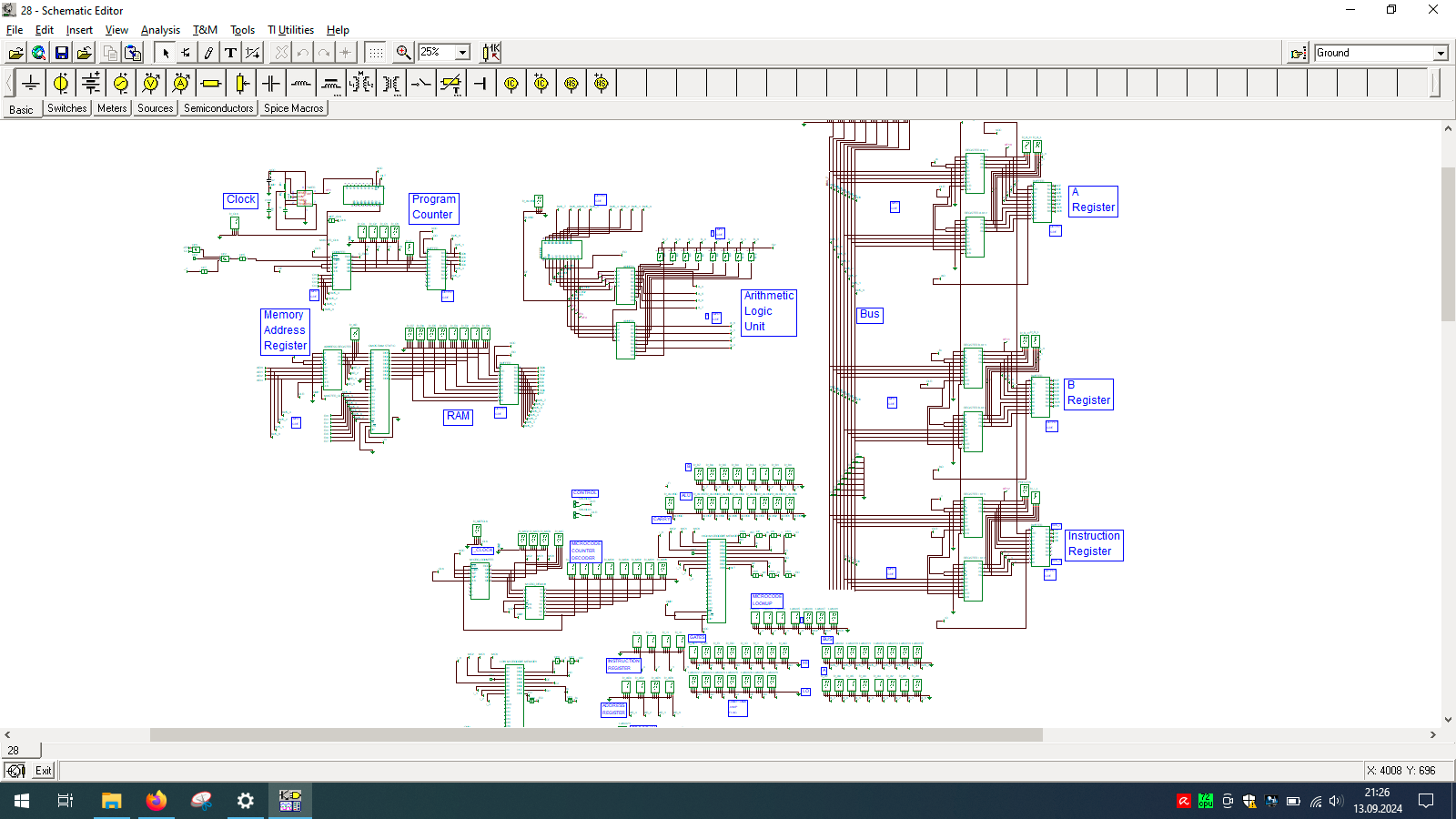
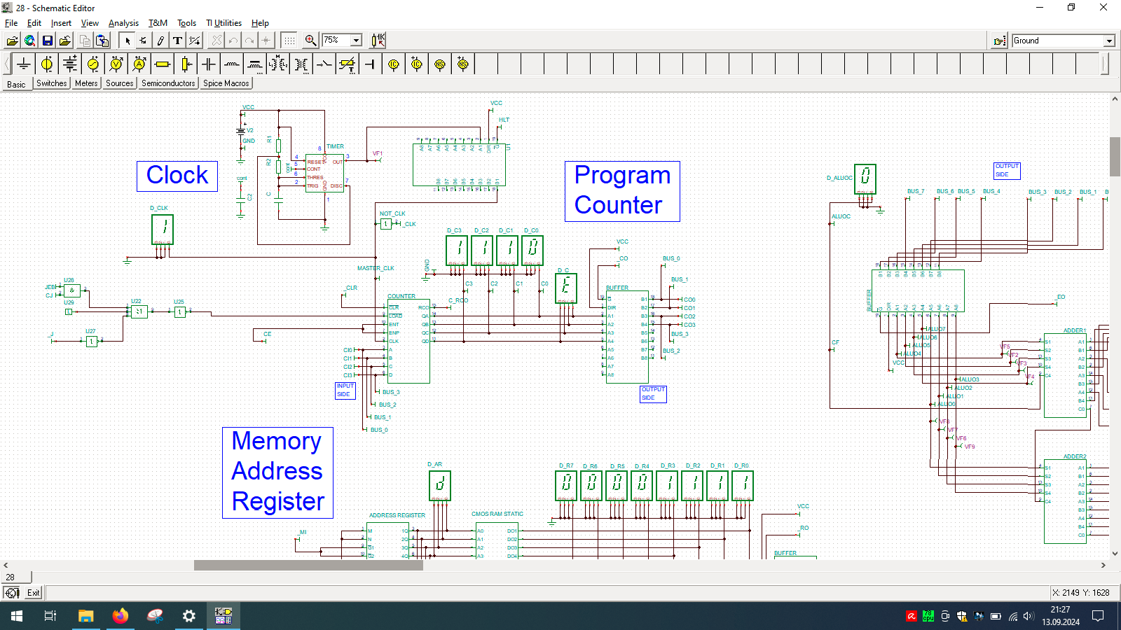
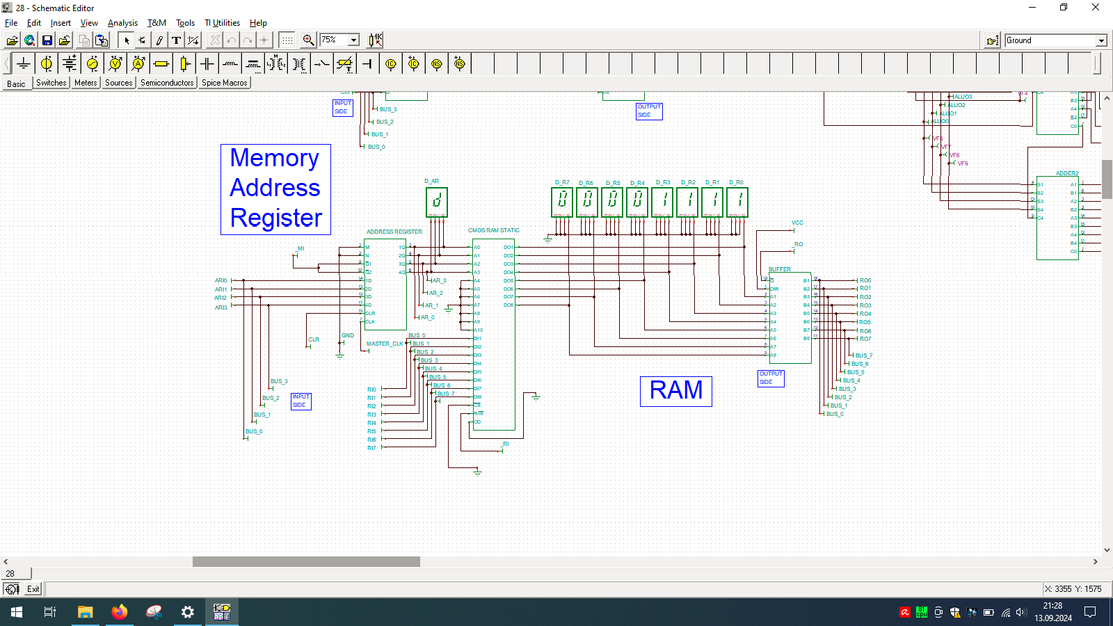
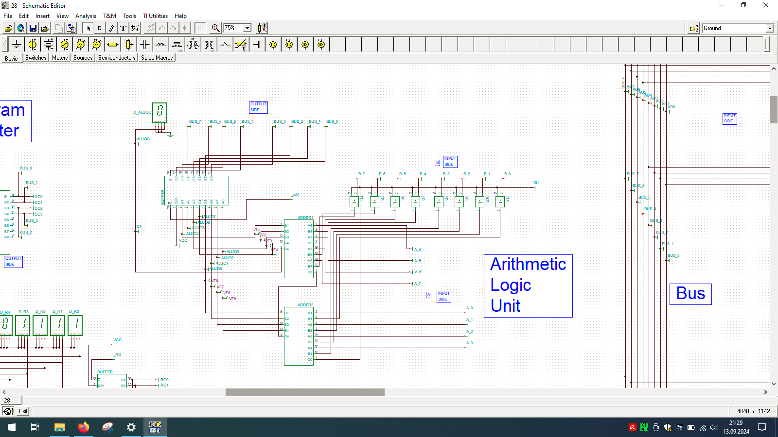
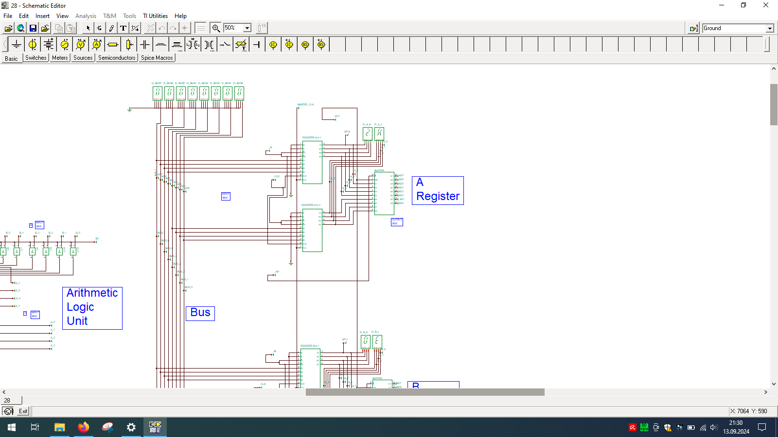
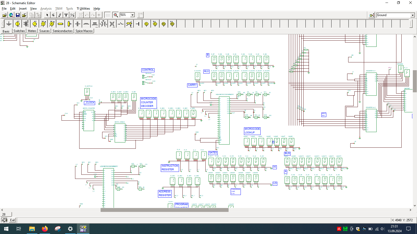
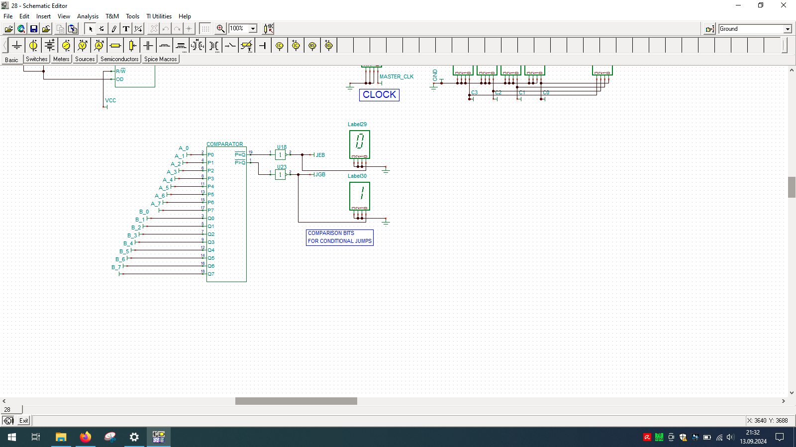
Even wondered how computer is built? And no, I’m not talking about unscrewing your laptop… but exactly how the things happen inside the CPU. If so, then check out TINA from Texas Instruments and open my custom-made all-in-one computer.
I spend few weeks preparing this schematic. It contains clock, program counter, memory address register, RAM, ALU, A&B registers, instruction register, microcode decoder, instruction register, address register and program counter. Well that’s a lot ot stuff you need to build 8-bit data and 4-bit address computer, even in simulator.
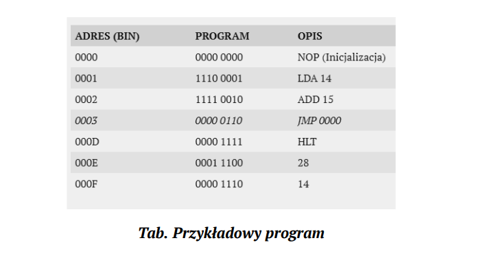
Sample program in my assembly + binary representation, which needs to be manually enter into memory in the simulator as there is input and output device designed for this machine. You need to program directly into memory and read its results also directly from the same memory but in different region.
Imagine you would like run 2 x vCPU and 4 GB RAM virtual machine. Which service provider do you choose? Azure, AWS or Hetzner?
With AWS you pay 65 USD (c5.large instance… and by the way why this is called large at all?). You pick Microsoft Azure you pay 36 Euro (B2s). If you would pick DigitealOcean then you pay 24 USD (noname “droplet”). Choosing Scaleway you pay 19 Euro (PLAY2-NANO compute instance in Warsaw DC). However, with Hetzner Cloud you pay as little as 4.51 Euro (CX22 virtual server). How is that even possible? So it goes like this (converted from USD to Euro):
AWS: 59 Euro
Azure: 36 Euro
DigitalOcean: 22 Euro
Scaleway: 19 Euro
Hetzner Cloud: less than 5 Euro
With different offers for vCPU and RAM the propotion stays similar, especially in Microsoft Azure. Both Azure and AWS are big-tech companies which make billions of dollars on this offer. Companies like DigitalOcean, Scaleway and Hetzner cannot be called big-tech, because they are much narrower in their businesses and do not offer that high amount of features in their platforms, contrary to Azure and AWS which have hundreds of features available. Keep in mind that this is very synthetic comparison, but if you would like to go with that specific use case scenario you will see the difference.
Every platform has its best. AWS was among the first on the market. Microsoft Azure has its gigantic platform and it is the most recognizable. DigitalOcean, Scaleway and Hetzner are many more (like Rackspace for instance) are the most popular, reliable among other non-big-tech dedicated servers and cloud services providers. I personally especially like services from Hetzner, not only because of their prices but excellent customer service, which is hard to offer within Microsoft or Amazon. If you want somehow more personal approach then go for non-big-tech solutions.
Important notice: any kind of recommendations here are my personal opinion and has not been backup-up by any of those providers.
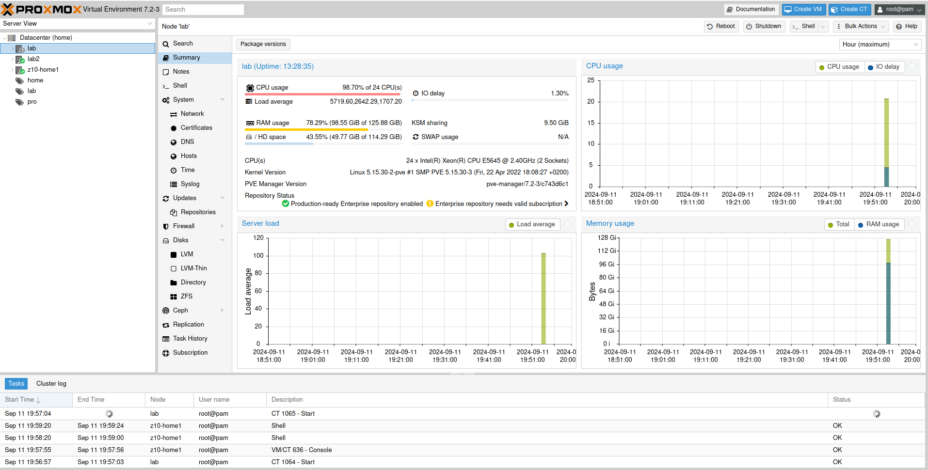
Ever wondered what can be the highest load average on the unix-like system? Do we even know what this parameter tells about? It shows the average number of either actively running or waiting processes. It should be close to the number of logical processors present on the system, otherwise, in case it is greater than this, some things will need to wait in order to be executed.
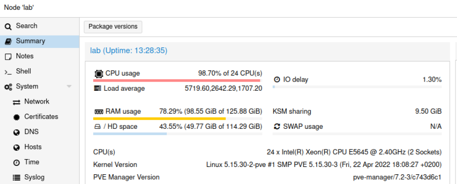
So I was testing 1000 LXC containers on the 2 x 6 core Xeon system (totalling as 24 logical processors) and leave it for a while. Once I got back I saw that there is something wrong with system responsiveness.
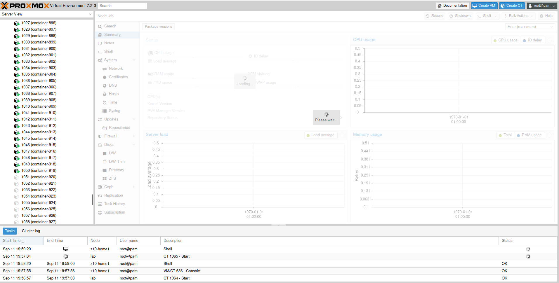
And my load average was 1min: 5719, 5 min: 2642, 15 min: 1707. I think that this the highest I have ever seen on systems under my supervision. What is interesing is that the system was not totally unresponsive, rather it was a little sluggish. Proxmox UI recorded load up to somewhere around 100 which should be a quite okey value. But then it sky-rocketed and Proxmox lost its ability to keep track of it.
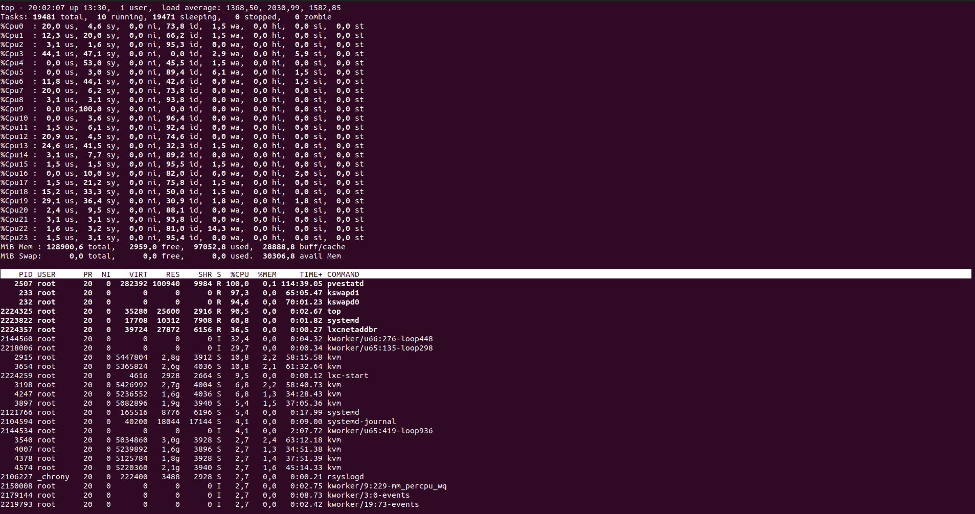
I managed to login into the system and at that moment load average was already at 1368/2030/1582, which is way less than a few minutes before. I tried to cancel top command and reboot it, but even such trival operation was too much at that time.
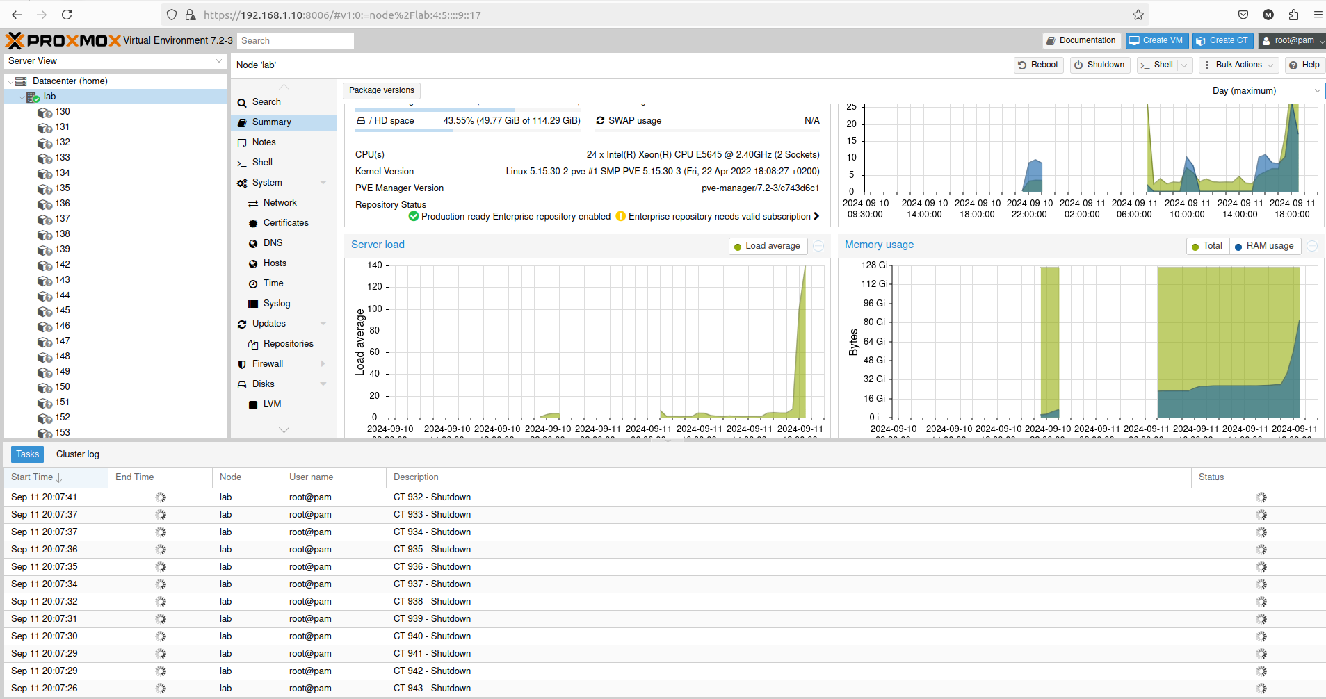
Once I managed to initiate system restart it started to shut down all those 1000 LXC containers present on the system. It took somwhere around 20 minutes to shut everything down and proceed with reboot.
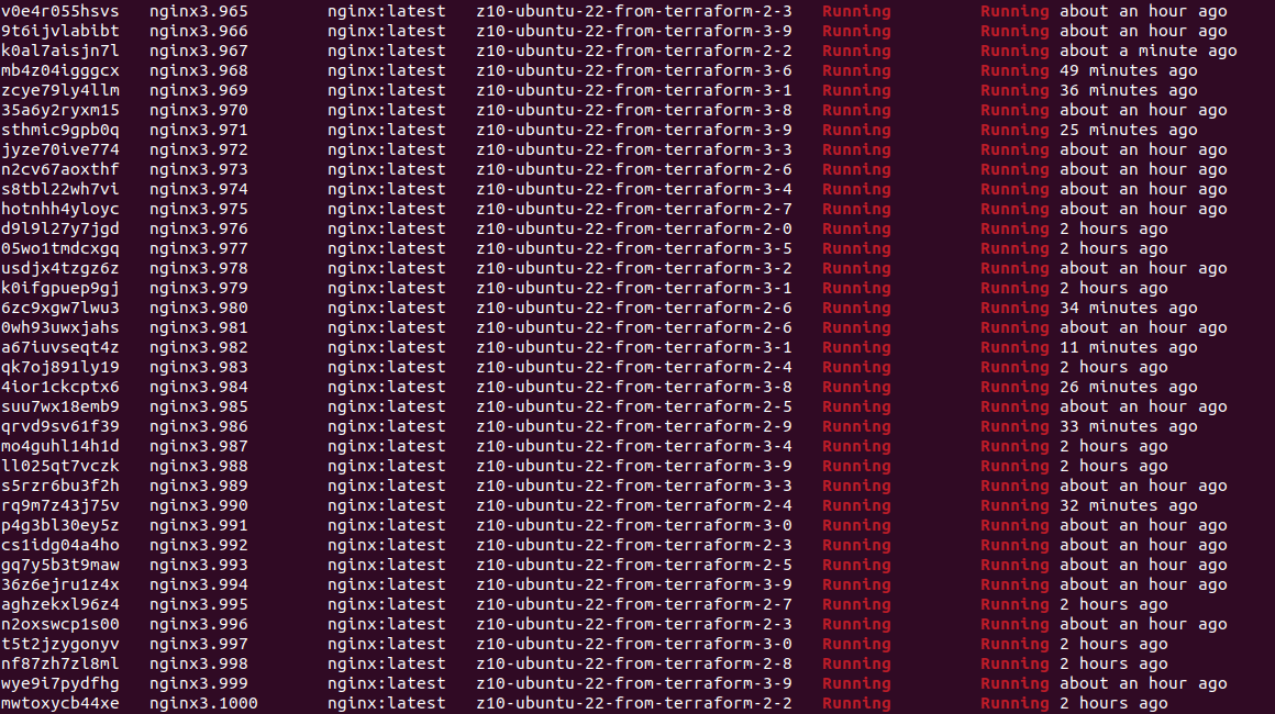
I defined Docker Swarm cluster with 20 nodes and created service using Nginx HTTP server Docker image. I scaled it to 1000 container instances, which took a while on my demo hardware. Containers are up and running but to get such statistics from Portainer CE UI is quite difficult, so I suggest using CLI in such a case:
docker service ps nginx3 | grep Running | wc -l
I got exacly 1000 containers on my service named “nginx3”.
Hardware is not so much utilized, combined 2 servers RAM usage oscillates around 50GB, load stays low as there is not much happening, so even using 20 VM and Docker containers, we do not get too much overhead of using both virtualization and containers. What about trying to spin 2000 or even 10 000 containers… Well, actually without putting load on those containers, measuring it will not be too much useful. We can scale even up to 1 000 000 containers, but what for?