The nature of wireless networking is quite problematic because transmission goes over air and can be intercepted by anyone. Of course there is data packet stream encryption. But deauthentication frames are not encrypted and can be forged. It’s applicable to IEEE 802.11 standard. However if your device is capable of 802.11w standard amendment then the management frames are protected from forging, however in various devices this option is disabled by default even if they support it. In case of your device check manual for default settings. It’s worth enabling this option. Not enabling, and securing both stations and base stations can lead not only to service denial/disruption, but also opens way to few possible attacks like “evil-twin“.
How to
To identify network or device to disrupt you can use airodump-ng. It turns your network adapter into listening mode and scans nearby networks. To switch between stations or base stations mode press “a”. For realtime sorting press “r”. Last must know shortcut is “s” for sorting. Space bar pauses scanning.
ip addr # to look for yournetadapter
sudo airodump-ng yournetadapter -w capturefilename
Base stations, which are access points are identified by column BSSID. Stations, which are clients, shows in the second table below. You can choose to deauthenticate just with MAC address of an access point or ESSID, which is human readible name. You can also pick some stations from the the second table to direct a deauthentication attack more precisely.
For a deauthentication part of the procedure use aireplay-ng tool. Pass –deauth with number of frames to send. If targeting only access points then pass -a with MAC of BSSID. If you target also some stations, then pass -c with MAC of a station (client).
sudo aireplay-ng --deauth 100 -a BSSIDMAC -c STATIONMAC yournetadapter
With proper values passed, stations will be disconnected from access point so their wireless service will be disrupted. As mentioned before it applies only to devices without IEEE 802.11w extension, which is most of consumer network devices. For enterprises it is highly possible that they will have proper enhancements already enabled.
Afterword
With airodump-ng you can select particular wireless channel to scan. You can also identify networks without security enabled at all. With traffic capturing feature enabled you can intercept precious parts of authentication procedure so you could try to crack it offline.
As an optional tool for any wireless related activities I can recommend WIFiman for Android which does the job of network perimeter exploration.
To provide security in a network you can deploy IDS or IPS systems. The difference is on the second letter, D stands for detection and P for prevention. First you start a system in IDS mode and only then you configure it to become IPS system. Enabling Suricata in IPS mode from the start could be confusing. It is advisable to see what’s going on first on a network to be sure not to generate too many false-positive alerts and blocks.
Fig. Traffic diagram
Why IDS/IPS?
You may ask why do I need intrusion detection or prevention system. It is a valid question because you may not want to know what is going on in your network or what malicious traffic is hitting your servers. But if you care about your data especially, then you should have such a system. In certain scenarios it might help lowering bad quality traffic as well.
About pfSense itself
I’m a great fan of pfSense since I think 2017. I’ve been using packet filter before and have been looking for user interface. Fortunately I found pfSense to meet my requirements. It contains firewall and router by default but can be enhanced by various packages like HAProxy, OpenVPN or IPsec.
Suricata installation & configuration in IDS mode
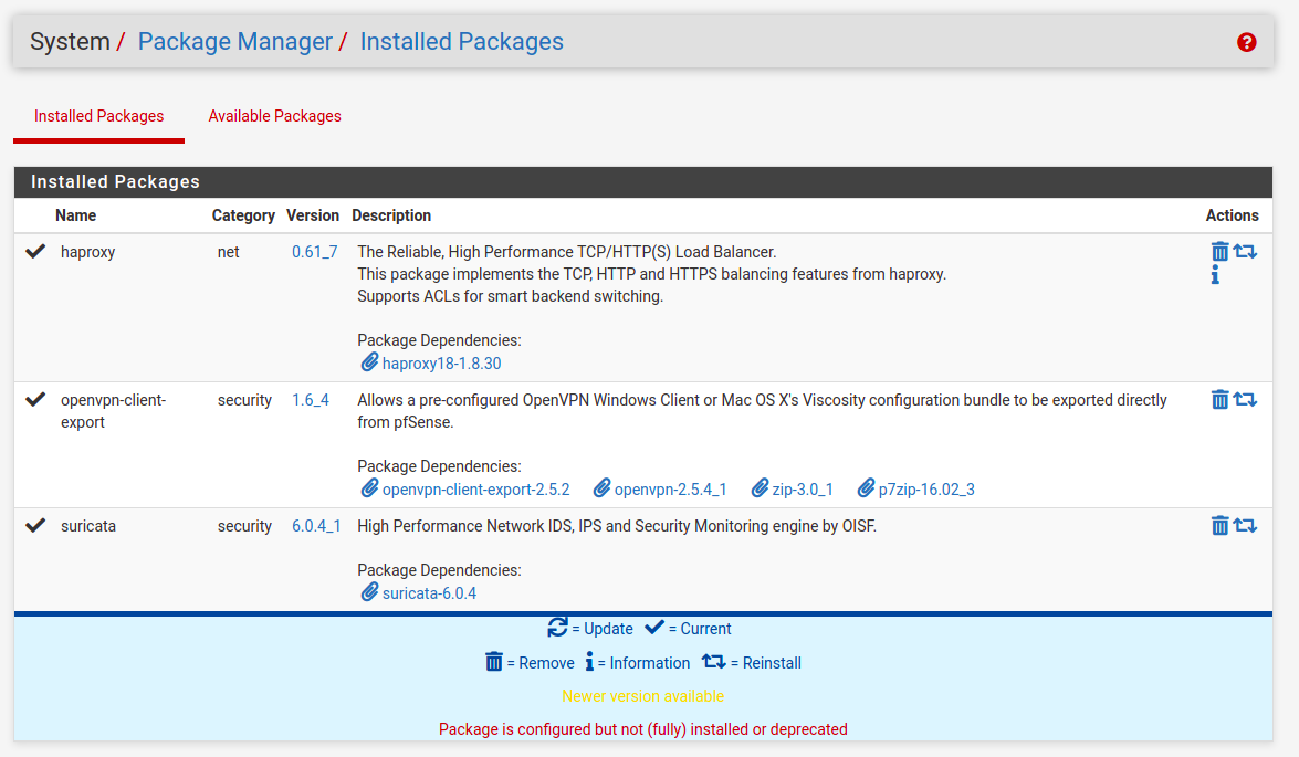
This IDS/IPS system can be installed as a standalone package without pfSense of cource, but it is especially useful when using together with firewall/router installation. The package can be found in pfSense’s package manager under System, Package Manager, Available Packages:
Fig. pfSense Package Manager
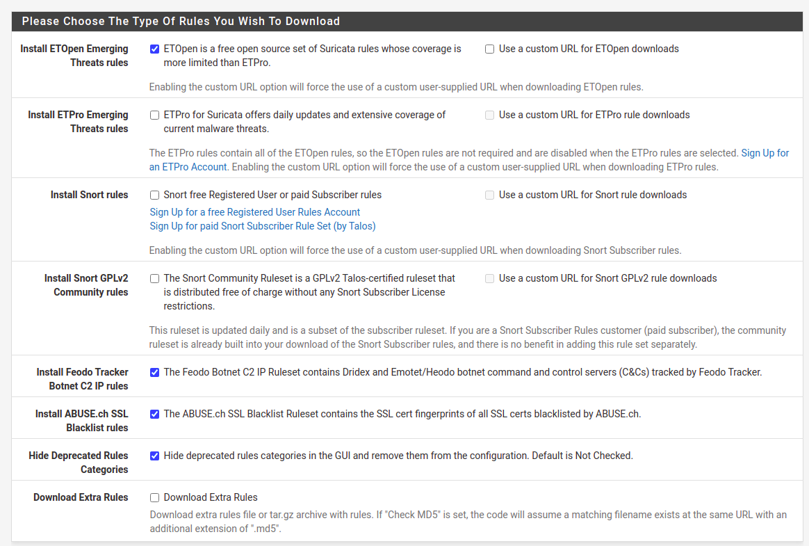
After installation, Suricata configuration page can be found under Services menu. You can with Global Settings first. Check “Install ETOpen Emerging Threats rules“, “Hide Deprecated Rules Categories”.
Fig. Rules download configuration
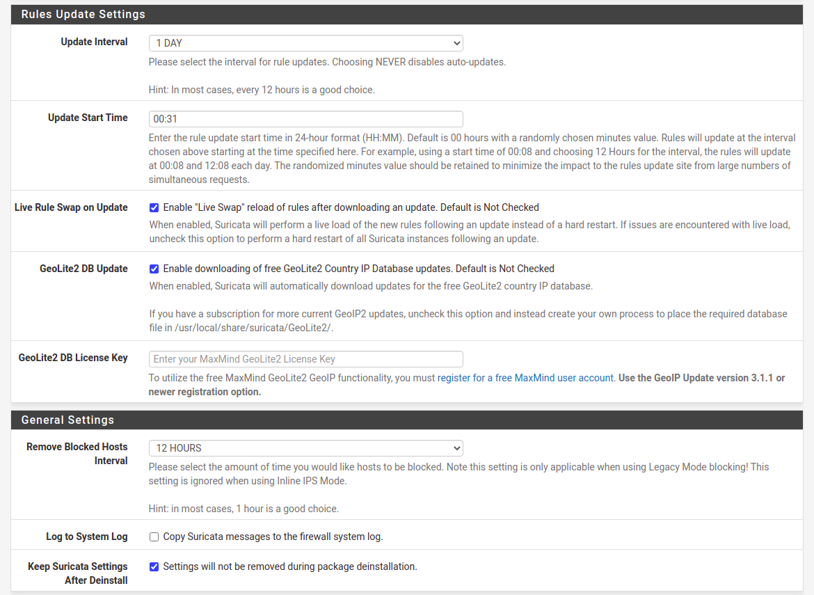
Below, select desired update frequency in “Update Interval” drop-down field. I select “1 DAY”. You can also check “Live Rule Swap on Update”, which will try to reload rules instead of just restart the service.
Fig. Frequencies configuration
For “Remove Blocked Hosts Interval” I select from 6 to 24 hours depending on the system specifics. Even if you will not start in IPS mode, be sure to check this at first configuration. It’s better to do this now instead of remembering to go back here after some time. You may just forget about it.
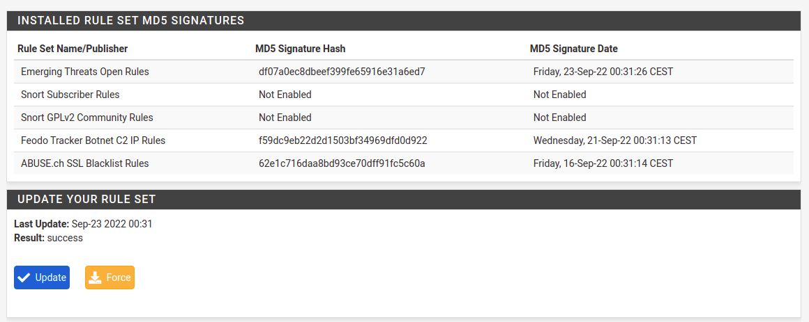
Next you need to force download rules in Updates tab. It does not trigger automatically for most of the time, so at first chance hit the Update button here.
Fig. Downloading rules
In case you have outdated pfSense installation there is high chance that the package will be outdated also and will try to download inexistent rules. It will end up with an error. I will not describe how to upgrade pfSense here, it will be covered in separate article. If rules download works just fine, then you’re fine, if it’s not, then prepare for some additional work.
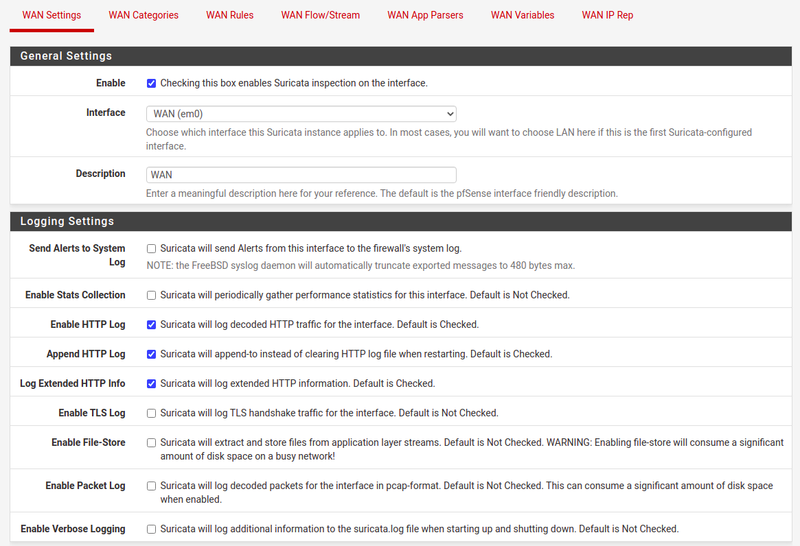
Next thing is to setup interface configuration. For to Interfaces tab and add an interface. There are few things to select there, starting with Enable checkbox if you want Suricata to run on this interface.
Fig. Interface general settings
You can try various options here for TLS, file-store and packet log. Except for TLS, the other onces, does require loads of disk space in a busy network. So remember to allocate enough storage here. There is one more thing in this section to configure, it is “Detect-Engine Profile”, which usually I set to “High” instead of default “Medium”. For now you do not select to block offenders, at first we stay as IDS intead of IPS mode.
For selecting only particular rules categories there is separate article (can be found under this link), so let me skip this one. For testing purposes I suggest enabling “3coresec”, “compromised” and “scan” rules categories. If done then go to Interfaces tab and restart Suricate on this interface. In case it is not starting, go to Logs View tab and browse suricata.log for some debugging information. Most of the time there is an issue with memory size versus configuration at Flow/Stream tab, but this is a subject for different article as well.
Enabling IPS mode
To prepare for prevention mode first go to Alerts tab and browse it for a while. Depending on a scenario you could spend 1 day or even a month just trying to understand what is going on your network/networks. For corporate networks there will be outgoing traffic more interesting that an incoming one. For service providers it is the opposite, so incoming traffic is the one to look after.
It is good to remember, that pfSense Suricata package will add your local network addresses, interfaces addresses and even tunnel subnets to pass list preventing them from blocking. In case you may want to block some internal addresses be sure to check this default pass list or even create your own one.
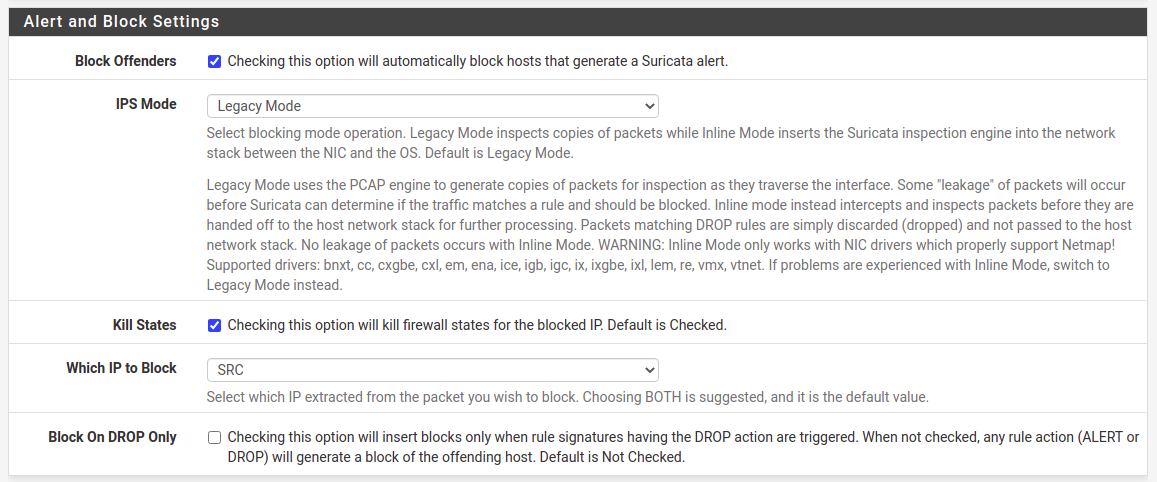
Once you have spent some time investigating what is going on within your network and incoming traffic as well, then it’s time to enable blocking mode. Go to interface settings and check “Block Offenders” option.
Fig. Enabling IPS mode, which blocks offenders
I prefer two things. First one is to select IPS Mode as “Legacy Mode” which copies packets instead of intercepting them between NIC and OS. It’s just simple for starters as there is little additional work to do opposite to “Inline Mode”. Second option I prefer is to block only source addresses, “Which IP to Block” set to “SRC”.
In case for outbound traffic a source address will be a local one, but it will not blocked because it is present on home network pass list. As I mentioned before, configuration depends on the characteristics of your networks you want to monitor. If you have more outgoing traffic then consider blocking target address. For some reason it is recommended to block both source and target, destination addresses. I am not sure exactly why as it clearly does not fit in all the cases.
Threats analysis
After configuration save, restart Suricata service on the interface and wait a while. Public IPv4 addresses are well known, so do not be surprised as within few minutes you will be scanned and explored by some kind of software crawlers. It is applicable even on newly assigned public addresses. For most installations I see from 50 to 500 blocked public addresses within one day of Suricata operating. For home and office networks you are going to see connectivity and updates checking from various devices. For enterprise setups traffic will be different and as it is broad topic it will be covered by another episode. So stay tuned.
Note: for more resilent setup install more than one Elasticsearch server node and enable basic security. For sake of clarity I will skip these two aspects which will be covered by another article.
Now be sure to configure both Elastic and Kibana. For Elastic it is /etc/elasticsearch/elasticsearch.yml configuration file. Be sure to set the following (change 0.0.0.0 with your local IP address):
sudo systemctl enable kibana
sudo service kibana start
Be sure to check if both Elasticsearch and Kibana are up and running with service or systemctl. If everything is fine proceed to setup Filebeat, Packetbeat on client hosts. There is separate guide how to do this. In beats configuration file point to Elasticsearch server you just installed.
HAProxy on pfSense
Example setup includes gateway, which is pfSense with HAProxy package. Configure two frontends, one for HTTP at 80 and one for HTTPS at 443. On HTTP frontend configure
Action http-request redirect
rule: scheme https
On HTTPS configure certificate and check SSL Offloading. Of course you need to load this certificate in System, Cert. Manager. Configure your backends and select it on HTTPS frontend. Now, go to HTTPS frontend and check the following:
Use "forwardfor" option
It is required to be able to read client IP in backend NGINX.
Filebeat on client host
On client hosts install filebeat package. There is separate guide for this one. Edit configuration file, which is /etc/filebeat/filebeat.yml:
filebeat.inputs:
  enabled: false
And then setup and enable NGINX module:
filebeat setup
filebeat modules enable nginx
Now, you are good to go with delivering log files, but first you need to point them in the configuration at /etc/filebeat/modules.d/nginx.yml:
You can use it in application configuration file at /etc/nginx/conf.d/app.conf in the server stanza:
access_log /var/log/nginx/app.log mydefault;
Restart your NGINX server and go to Kibana to explore your data. You need to add this log format, in order to handle client IP which is present in $http_x_forwarded_for variable. This format as close as possible to the default one.
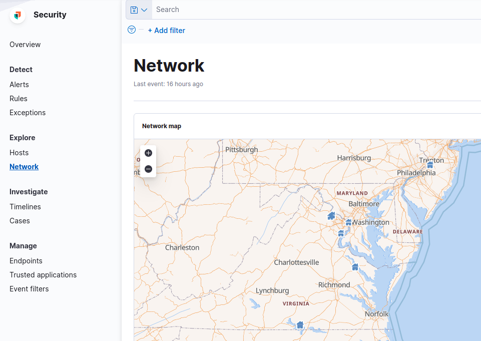
Network geo location map
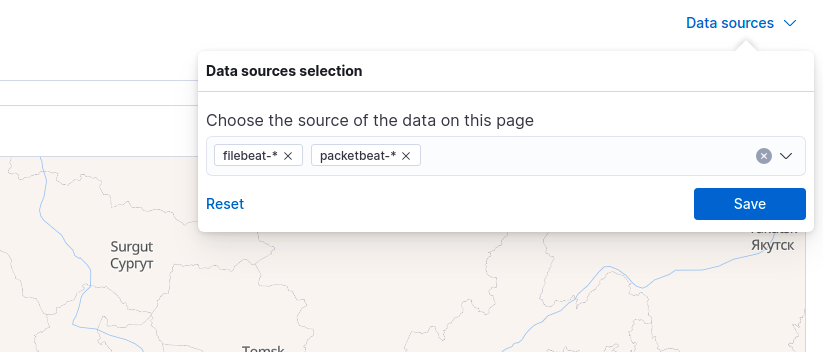
If everything went fine which is installting Elasticsearch, Kibana, beats on your client hosts and configuration of HAProxy, NGINX, then you can open Security, Explore, Network section and hit refresh buton to load data into map. But first you need to select Data sources (link above the map, on the right side), include filebeat-* index pattern.
Fig. Filebeat data source selection
With such configuration you should be able to see geo points representing client locations.
Fig. Location points based on filebeat data
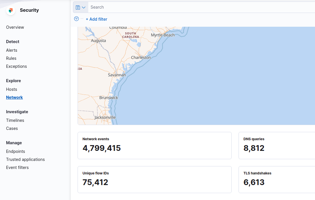
In case you also enable Packetbeat, you will see also networking information data below the map.
Fig. Networking information data
Please remember that enabling Packetbeat generates tons of data in complex environments, so be sure to allocate enough space for these indices.
Summary
This guide covers the basic path for installting Elasticsearch, Kibana, Beats and configuring HAProxy and NGINX to deliver traffic, logs to Elasticsearch and be able to visualize traffic as geo location points.
Among 3 million public IP address ranges for the whole world, 68k belongs to the Russian Federation. This translates into 45 million addresses. Scanning the HTTP port on this population took 20 hours. I obtained 630k IP addresses with listening on port 80. Of which 530k gives the correct answer of the HTTP type. Only 340k gives an HTTP 200 response. Over 200k run on NGINX servers, and 100k run on Apache. When analyzing the content, you will find GitLab, Kibana, Zabbix or Grafana installations open for registration and use, but also copies of databases, video surveillance systems, etc. My favorite find, however, is the control panel of the heat plant…
When I bought the HP z800 workstation at the beginning of 2021, I wanted to increase my competences in the field of hardware and software optimization on the one hand, and on the other hand, describe it in the form of a publication in order to consolidate my knowledge sufficiently. Over the course of the following months, the concept changed dramatically, and I needed more information. I decided that I needed to expand my knowledge of hardware construction. The final part of this was the development of the concept of a series of notebooks entitled “Simple High Performance Computing“, or HPC in an edition available basically for everyone in every budget.
6 parts are planned in the series, 2 have already been completed and released
The first part of the series is “Fundamentals of electronics and building a computer in a simulator” published in 2021 (available for download at this address). The second part (number 5 in the series) was “OpenCL, CPU and GPU programming” released in May 2022 (available for download at this address). In addition to these two items, the series also includes parts for the review of computer platforms from the 1980s to now, including MOS 6502, Intel SSE, AltiVec, OpenGL and possibly ESP8266. The last part is “Data Mining & Exploration“, which is the subject of this particular article.
Target group
Using the ip2location database to scan the selected territory
I take a few services as an example for data mining, but I’ll start with the basic ones, HTTP and DNS . I identify the target group using the ip2location database. It is a collection of ranges on the public internet with information about the belonging to a given territory. Today we have 2 975 657 pieces of all IPv4 Internet ranges. Loaded into PostgreSQL 14, they take 405 MB. In the ip2location database, the ip2location_db11 table stores ranges of public IPv4 addresses. It is the broadest free collection containing granularity of locality and approximate location data . There is also a zip code here. Of course, in the case of larger towns and cities, there may be many such codes.
Note: ip2location database is also available in commercial version, where we get additional metadata and geolocation is much more precise. The database has ranges for 242 territories. Interestingly, the World Bank’s WDI database defines 265 territories, and there are 193 members of the United Nations. Both databases try to follow the letter of the law regarding the recognition of individual countries. So even if a territory is dependent on another country, but it is generally recognized, such territory will have separate data, for example, Nothern Mariana Islands. However, we will not find the Republic of Artsakh or Kosovo.
Tools
For exploration, I use zmap, dig and an application written in Ruby
The zmap program is designed for high-performance scanning of network spaces. It is assumed that on properly selected equipment and Internet connection, you can scan the entire IPv4 space within a few hours on a selected TCP port. Of course, this type of mass scans can put your address on the fraud lists and be de facto blocked in many places around the world. There are two strategies to avoid this. The first is to use a separate space for such scanning, e.g. a virtual machine in a public cloud (DigitalOcean, Rackspace, Microsoft Azure, etc.). At the beginning of my adventure with this type of scans, I chose this option myself. After informing the supplier about the scheduled scanning, we should not have any problems, it is only worth mentioning that these are research works. The second strategy I am currently using is scanning at lower bandwidth, clearly defined regions in the world. The downside of this solution is, of course, lower efficiency, resulting from the need to operate on CIDR blocks that are usually not adjacent to the networks so that they can be merged. Not being able to randomize scanning is a major drawback.
As for dig , I use it to test DNS server responses, but also as a reverse IP address to domain name mapping tool for the entire address population. Domain analysis for HTTP services is interesting, but it is more interesting to map domains for all IP addresses, but it requires the use of more DNS servers so as not to be blocked on the most popular ones.
The whole, i.e. both zmap and dig based tasks are merged using an application I called miner, made in Ruby and Ruby on Rails , used for orderly execution such operations step by step. Basically the app only uses ActiveRecord , Rake and HTTParty so it’s a bit exaggerated to say that this is a Rails app. For more demanding operations, I use dedicated modules and methods for HTTP connections, because HTTParty has various limitations and errors that easily come to the surface at such a scale. The same goes for the Parallel library, which is obviously invaluable in the context of concurrent work, removing the need for the user to work directly on threads and processes, but has a number of unresolved bugs and memory leaks.
Note: if I find some free time, I will try to repeat long-distance attempts to reveal memory problems of the libraries, so I will have an evidence to report bugs to their creators .
Hardware
Paradoxically, mass scanning does not require too powerful equipment
As I mentioned in the introduction, I use the HP z800 workstation for this work, which accepts a maximum of 2 CPUs, each with 12 threads, for a total of 24 logical processors per station (Intel Xeon X5660). I used two of such workstations for the test, so I had 48 processors in total. As for the operating memory, the maximum for such a set is 768 GB DDR3, although I only have 180 GB installed. Scanning and the activities around it are not memory-intensive, they require a large amount of CPU and a stable network on the hardware and network software layer. I used my 1 Gbps downlink and 600 Mbps uplink to scan. The network traffic is managed by the installation of pfSense 2.6 on dedicated hardware with the Intel Xeon E3 1230 processor. At the peak of the scan, the number of states on the firewall reached 500,000, which was due to the liberal configuration. With a bit more strict control of states, the number can be significantly smaller, but then we increase the risk of closing good states.
Note: Scanning can generally be performed on any hardware with a decent network card. What is meant by decent? First of all, it should be a minimum 1 Gbps card, and preferably with a speed of 10 Gbps. It should be made by a reputable manufacturer. It should also be a popular model with a current firmware available.
Loading addresses
Translate ranges to proper IPv4 public addresses
The procedure begins with the conversion of IP ranges in CIDR notation to the proper atomic IP addresses. Since ranges are represented numerically, we can use Ruby’s Range class to do this:
The actual task generating addresses from ranges is as below. Originally, this task was adapted to generate addresses from ranges for countries with an allocation of less than 5 million addresses, there are about 200 such territories.
  desc "Generate and insert IP list based on IP2Location IP ranges"
  task :generate_ip_list_from_ip_range => :environment do
    sql = "SELECT country_code, SUM(ip_to-ip_from) AS cnt
            FROM ip2location_db11
            WHERE country_code IN
              (
                SELECT DISTINCT a.country_code
                FROM ip2location_db11 a
                LEFT JOIN servers b ON a.country_code = b.country_code
                WHERE b.country_code IS NULL
              )
              AND country_code = 'RU'
            GROUP BY country_code;"
    res = IpAddress2.connection.execute(sql) # ip2location_db11
    res.each do |r|
      puts r.inspect
      ranges = IpAddress2
                .where("country_code = ?", r["country_code"])
                .select("'0.0.0.0'::inet + CAST(ip_from AS bigint) AS mfr,
                         '0.0.0.0'::inet + CAST(ip_to AS bigint) AS mto,
                	  country_code, country_name, region_name, city_name,
                          latitude, longitude, zip_code, time_zone")
      ranges.each_with_index do |range,index|
        puts "from: #{range.mfr}, to: #{range.mto}"
        if !range.mfr.blank? && !range.mto.blank? then
          ips = convert_ip_range(range.mfr.to_s, range.mto.to_s)
          elements = []
          cnt = 0
          ips_size = ips.size
          puts " ips_size: #{ips_size.to_s}"
          ips.each_with_index do |ip,index2|
            s = Server.new
            s.ip = ip
            s.country_code     = range.country_code
            s.geo_region_name  = range.region_name.gsub("'", "")
            s.geo_city_name    = range.city_name.gsub("'", "")
            s.geo_latitude     = range.latitude
            s.geo_longitude    = range.longitude
            s.geo_zip_code     = range.zip_code
            s.geo_time_zone    = range.time_zone
            cnt = cnt + 1
            elements << s
            if cnt >= 500 || index2+1 == ips_size then
              puts " #{cnt.to_s}: importing #{elements.size.to_s}"
              Server.import(elements, returning: :ip)
              elements = []
              cnt = 0
            end
          end # ips
        end # if blank
      end # IP ranges
    end # SQL res
  end # task
The range generation has several imperfections. The final number of the resulting addresses is greater than that declared by ip2location and it is not due to the generation of subnet and broadcast addresses. However, this is of little importance in the overall scale. Generating in this form takes several hours depending on the adopted size of the batch package (500, 1000 or other).
zmap scanning of HTTP servers
Quantitative qualification using zmap
There are two approaches to performing a scan and it is not about distinguishing whether we are scanning from a location other than ours or scanning at a slow pace. It’s about the launch mode. We can scan in series or in parallel. Serial scanning is slow and range merges are difficult to accomplish in a short time. We can try to merge smaller ranges (subnets / 24) into larger ones (e.g. / 16) using the Ruby NetAddr module:
result = NetAddr.summ_IPv4Net(cidrs)
Unfortunately, the code of this module is suboptimal and fails to execute properly due to memory error, cavities and overall huge processing time. Perhaps someday I will find a moment to write an alternative, but the problem is only apparently simple. In any case, in order to generate a CIDR range from a numeric range, we again need the code snippet as below:
 def iprange2netmask(ipstart, ipend)
    if ipstart.kind_of?(String) || ipend.kind_of?(String)
      startR = ip2long(ipstart)
      endR = ip2long(ipend)
    else
      startR = ipstart
      endR = ipend
    end
    result = Array.new
    while endR >= startR do
      maxSize = 32
      while maxSize > 0 do
        mask = (iMask(maxSize - 1))
        maskBase = startR & mask
        if maskBase != startR
          break
        end
          maxSize-=1
      end
      x = Math.log(endR - startR + 1)/Math.log(2)
      maxDiff = (32 - x.floor).floor
      if maxSize < maxDiff
        maxSize = maxDiff
      end
      ip = long2ip(startR)
      netmask = cidr2netmask(maxSize)
      cidr = [ip, netmask].join('/')
      result.push("#{ip}/#{maxSize.to_s}")
      startR += 2**(32-maxSize)
    end
    return result
  end
  def iMask(s)
    return (2**32 - 2**(32-s))
  end
  def long2ip(num)
    return IPAddr.new(num, Socket::AF_INET).to_s
  end
  def ip2long(ip)
    return IPAddr.new(ip).to_i
  end
  def cidr2netmask(cidr)
    IPAddr.new('255.255.255.255').mask(cidr).to_s
  end
Having a ready method for translating a numerical range into a CIDR range, we can generate scanning scripts using the following task. The task creates the necessary directory structure where the scripts using the zmap program will be placed. The parameters used for scanning are 100 Mbps bandwidth and 2 attempts. In the zmap configuration in the /etc/zmap/zmap.conf file, I also indicated the waiting time for the response in the cooldown-time parameter of 2 seconds.
 desc "zmap to port X"
  task :generate => :environment do
    port = 80
    countries = Server.all
                  .select("country_code, count(*) AS cnt")
                  .group("country_code").order(Arel.sql("COUNT(*) ASC"))
    countries.each do |c|
      puts "#{c.country_code}: #{c.cnt}"
      ranges = IpAddress2
                 .where("country_code = ?", c.country_code)
                 .select("'0.0.0.0'::inet + cast(ip_from AS bigint) AS mfr,
                          '0.0.0.0'::inet + CAST(ip_to AS bigint) AS mto, country_code")
      if Dir.exist?("/opt/repos/zmap/#{port}/{c.country_code}") then
        next
      else
        FileUtils.mkdir_p("/opt/repos/zmap/#{port}/#{c.country_code}")
        FileUtils.mkdir_p("/opt/repos/zmap/#{port}/#{c.country_code}/scripts")
        FileUtils.mkdir_p("/opt/repos/zmap/#{port}/#{c.country_code}/scripts/done")
        FileUtils.mkdir_p("/opt/repos/zmap/#{port}/#{c.country_code}/results")
      end
      ranges.each_with_index do |range,index|
        path = "/opt/repos/zmap/#{port}/#{c.country_code}/scripts/run_#{range.mfr}_#{range.mto}.sh"
        iprange2netmask(range.mfr.to_s, range.mto.to_s).each_with_index do |cidr,index2|
          puts "RANGE: #{range.mfr} do #{range.mto}"
          command = "zmap --bandwidth=100M --target-port=#{port}
           --output-file=/opt/repos/zmap/#{port}/
                         #{c.country_code}
                         /results/#{range.mfr}_#{range.mto}.csv
           --probes=2 #{cidr}\n"
          File.write(path, command, mode: "a")
        end # cidrs
        command2 = "ping -c 1 1.1.1.1\n"
        File.write(path, command2, mode: "a")
        command3 = "if [ $? -eq 0 ];
                    then mv #{path} /opt/repos/zmap/#{port}/#{c.country_code}/scripts/done;
                    else echo '!';
                    fi\n"
        File.write(path, command3, mode: "a")
      end # ranges
    end # countries
  end # task
Regardless of how we run the task, whether in series or in parallel, we will face the same problems when it comes to completeness of the results obtained. We are talking about waiting time for an answer. By default, zmap uses up to 8 seconds of waiting, which means a lot of delays with many subnets with the CIDR / 24 mask. Scanning 256 hosts (minus the network address and broadcast address) takes a blink of an eye, so the subsequent waiting of 8 seconds is definitely redundant here. At the same time, if we set this parameter to 1 second, it may turn out that we lose correct answers that have not reached us due to delays on the backbone network or even on our local network.
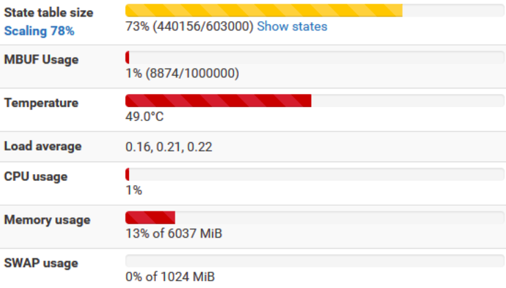
If we don’t want to aggressively optimize the pfSense configuration in terms of state performance, then we have to increase the RAM memory so that all the redundant states fit. You need at least 4 GB to be able to start such a scan. Anything above increases the possibilities, and 16 GB is preferable. By the way, we will have the opportunity to know, as well as I, that pfSense has special optimization mechanisms when there are a number of states above certain thresholds.
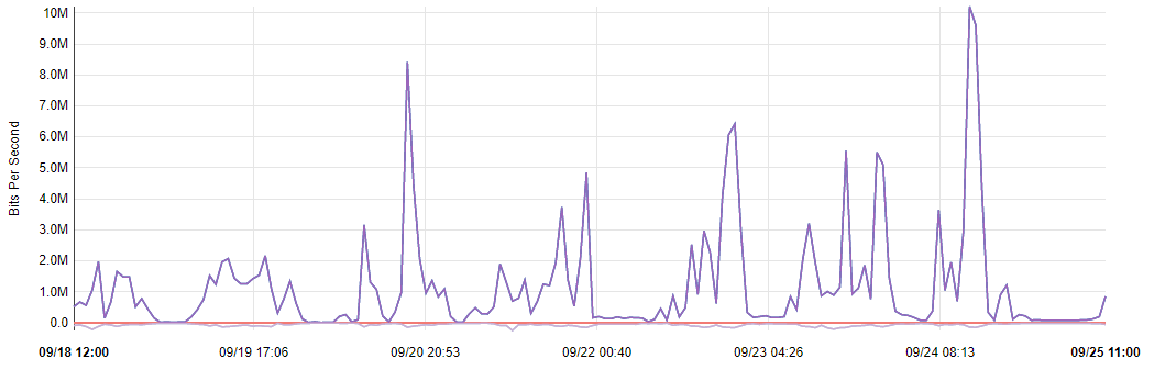
Fig. Scaling the state table at high traffic saturation
Parallel processing was achieved by using the Parallel library. By trial and error, I determined that with 6 GB of memory, it would be optimal to use 4 processes. I also tried higher values, e.g. 16 processes, but I would have to install 16 or even 32 GB of memory into pfSense. It could also have a negative impact on the use of the local network as such. I used the following task for parallel processing.
  desc "run zmap in parallel"
  task :run => :environment do
    country_code = "RU"
    port         = 80
    scripts = Dir["/opt/repos/zmap/#{port}/#{country_code}/scripts/*"]
    Parallel.map(scripts, in_processes: 4) do |script|
      puts "#{Parallel.worker_number} => #{script}"
      system(script)
    end
  end
Scanning took 20 hours. During this time, zmap only sent 5 GB of data packets. 45 million atomic IP addresses were scanned from 68k ranges and 177k lowest order networks. The result is 630k addresses where listening on port 80. This does not mean that there are HTTP servers there, just that the server responds to packets sent by zmap. This is a quantitative qualification. In the last step, the results were transferred to the database, to a dedicated table based on the results.
Note: I know from my own experience that zmap scans can be detected using signatures in IPS / IDS applications such as Suricata. Perhaps, therefore, some hosts did not respond, because they detected in proactive mode that a zmap scan was being performed. What is certain is that a system of this kind may block further communication from the source address for some time. It is therefore a good practice to wait 24 hours before attempting qualitative verification on these hosts.
Qualitative verification
Analysis of content offered by remote hosts
I started working with HTTP servers by saying that on such a large population of hosts there is too much variation in protocol implementations that the use of a simple and convenient HTTParty library is insufficient. At first glance, I needed a dedicated method that wouldn’t make any far-reaching assumptions about the operation of the remote host. Here is the code.
module FetchUtil
  # Fetch a URL, with a given max bytes, and a given timeout
  def self.fetch_url url, timeout_sec=4, max_bytes=1*1024*1024
    uri = URI.parse(url)
    t0 = Time.now.to_f
    body = ''
    code = nil
    headers = []
    Net::HTTP.start(uri.host, uri.port,
               :use_ssl => (uri.scheme == 'https'),
               :open_timeout => timeout_sec,
               :read_timeout => timeout_sec) { |http|
      # First make a HEAD request and check the content-length
      check_res = http.request_head(uri.path)
      code = check_res.code
      raise "File too big" if check_res['content-length'].to_i > max_bytes
      # Then fetch in chunks and bail on either timeout or max_bytes
      # (Note: timeout won't work unless bytes are streaming in...)
      http.request_get(uri.path) do |res|
        res.each_header do |k,v|
          headers << [k,v]
        end
        res.read_body do |chunk|
          raise "Timeout error" if (Time.now().to_f-t0 > timeout_sec)
          raise "Filesize exceeded" if (body.length+chunk.length > max_bytes)
          body += chunk
        end
      end
    }
    return [code, body, headers]
  end # fetch_url
end # module
This code has two constraints, size and time. We limit the size to 1 MB of data and 4 seconds of waiting for the result. This is part of a larger task that is responsible for concurrent verification. The module described above is used, but also HTTParty, where there is a 3xx response code. I am also trying to convert the ASCII-8BIT to UTF-8 encoding, but this is a very extensive topic, especially that the selected territory does not use the Latin alphabet.
def perform_verify
    @reconnected ||= Server.connection.reconnect! || true
    port = 80
    Parallel.each_with_index(Server80.where("is_checked is false ")
            .limit((1024*64)), in_processes: ENV['PC'].to_i * 1) do |s,index|
      $stdout.sync = true
      @reconnected ||= Server80.connection.reconnect! || true
      puts "#{Parallel.worker_number}: #{index}: (#{ENV['PC'].to_i*1}): #{s.ip}: #{s.country_code}"
      start = Time.now
      begin
        resp     = FetchUtil.fetch_url("http://#{s.ip}:#{port}/")
        code     = resp[0]
        body     = resp[1]
        hdrs     = resp[2]
        if code.to_s[0] == '3' then
          puts " switching to httparty as 3xx"
          response = HTTParty.get("http://#{s.ip}:#{port}", timeout: 2)
          code = response.code
          body = response.body
          hdrs = response.headers
        end
        if true
          str = body
          enc = body.encoding rescue nil
          puts " #{enc}"
          if enc.to_s == "ASCII-8BIT" then
            str = body.force_encoding(enc).encode('utf-8', invalid: :replace, undef: :replace)
            str.scrub!("")
            str.gsub!(/[[:cntrl:]&&[^\n\r]]/,"")
          end
          doc = Nokogiri::HTML(str)
          s.headers  = hdrs
          s.content  = str
          s.csize    = str.size
          s.title    = doc.xpath("//title").text
          s.start    = start
          s.finish   = Time.now
          s.diff     = (s.finish - s.start).in_milliseconds
          s.result   = code[0..999]
          if    code.to_s[0] == '1' then
            s.is_1xx = true
          elsif code.to_s[0] == '2' then
            s.is_2xx = true
          elsif code.to_s[0] == '3' then
            s.is_3xx = true
          elsif code.to_s[0] == '4' then
            s.is_4xx = true
          elsif code.to_s[0] == '5' then
            s.is_5xx = true
          end
          puts " .. #{s.result} -#{s.result.size}- .. #{s.title} .."
          s.is_checked = true
          s.save!
        end
      rescue Exception => e
        puts " exception: #{e}"
        s.content = nil
        s.title = nil
        s.result = e.to_s[0..999]
        s.is_checked = false
        s.is_http_error = true
        s.save!
      end
    end # parellel
  end # task
I use Nokogiri and xpath selectors to process responses. When the task with 24 processes was running, the number of states on pfSense was from 30k to 40k. The combination of Parallel and HTTParty and closer to unknown hosts often causes processes to be blocked. It seems that the main culprits here are Parallel and its compatibility with other elements, because this behavior is also observed in other projects, where there is no HTTParty library used, but only ActiveRecord. There is an option of full process separation, but it causes a drastic drop in performance, which generally disqualifies this option. There is also another explanation that may explain this behavior in part. Well, some of the hosts offer streaming services which is difficult to identify. They might send fake HTTP metadata, but actually offer something completely different.
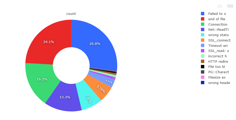
Moving on to the analysis of the results, the correct answer was sent by 522k hosts plus 8k hosts in the retry. This gives a total of 530k correct answers and 99k various types of connection errors on the HTTP protocol. I did 5 full runs to confirm that the failed hosts did indeed permanently offer no HTTP content. 16% of the hosts that answered port 80 are incorrect. The division among incorrect answers is as follows.
Fig. Detailed analysis of connection errors
“Failed to open TCP connection” is responsible for the biggest part of errors, 26.8%, 26398 items. Second in line is “end of file reached“, 24.1%, 23817 units. Third place is “Connection reset by peer“, 16.2%, 15986 units. Next are Net :: ReadTimeout, “wrong status line“, SSL_connect, TimeoutError, SSL_read, HTTP redirects, “File too big“. The remaining error messages are responsible for a small percentage and there are a lot of different types. They result from running non-HTTP services on port 80 and 443. Among correct HTTP responses, i.e. a pool of 530k hosts are divided into the following division.
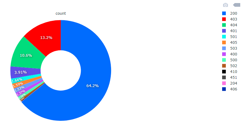
Fig. The division into codes of correct responses of HTTP servers
HTTP response codes are divided into 5 categories. Codes starting with 1 are info codes. Codes starting with 2 are correct answers. Codes starting with 3 are redirects of various types, additional action is required. Codes starting with 4 are client errors that prevent further processing of the request. Codes starting with 5 are server errors. The list of HTTP response codes is maintained by IANA.
HTTP 200 codes are 340k. We have codes 403 with number of 69k. We have 56k codes 404. We have 20k codes 401. The remaining group of a dozen or so types of answers is below 10k each of these types.
Analysis of the results
Configuration and content
We can consider the content offered by HTTP servers from several angles. First of all, it should be noted that when we talk about public IPv4 addresses, we are talking about either physical or virtual network adapters. In both cases, multiple domains may be running on a given host based on SNI. These hosts can and certainly act as entry points for a subnet (NAT or proxy). Of course, this does not apply to all addresses, only parts. What, it is not known. The analysis may concern the HTTP server as such, its type, version and configuration, or the content returned by this server. Both analyzes bring many interesting facts.
Configuration analysis
Operating systems and runtime platforms
When examining the configuration, I find that among all the answers, 217k hosts are supported by the NGINX server, 96k through the Apache server, and 20k by the Microsoft IIS server. The most popular HTTP servers are responsible for a total of 334k addresses. There are 7810 of all the varieties of the reported servers. The more interesting less popular servers are Webrick, Lotus-Domino or Mongrel, but also MinIO and WowzaStreamingEngine. There are also print servers, Couchbase and many more. From the series of these strange ones, I would single out “Aeroflot“, “Stalin” or the “ZX Spectrum“. However, to indicate something specific, I would say that it is NGINX 0.4.13 from 2006 or Phusion Passenger in an older version. In general, all older versions of HTTP servers may be subject to exploit tools.
Another aspect of the configuration study is the operating systems and runtime platforms on which the HTTP hosts and servers are running. Servers with a declared Windows system are 5257 pieces. By contrast, Ubuntu Linux is 52473 units, Debian is 16438 units. Among other popular systems, it is CentOS in the amount of 31176 units. The FreeBSD system is also popular with a total of 3326 units. The most popular technology stack we know about from the headers is PHP. It is not, however, that this information is confirmed, because basically only this language module is widely advertised, and the others are simply not. We will not find such information in the case of Java or Ruby languages. The exception will be the Perl as Apache module. It occurs in 662 pieces.
Information about the operating system or runtime platform, and in particular their versions, is important from the point of view of the security of such hosts. A Linux or FreeBSD host is just as vulnerable as a Windows host . This is because they can be misconfigured in the first place, and not so much vulnerable. Windows systems are much more popular from workstations than servers, hence the large majority of threats present on this system. When it comes to vulnerabilities, the first choice is metasploit, which will give us information whether the vulnerabilities on the hosts can be exploited.
Note: it is important to know that “Data Mining & Exploration” is about information and fact-finding, not security hacking and misconfiguration.
Content analysis
Systems and applications
In addition to the configuration of servers, we can examine what content they return. This allows us to get to know the specificity of the studied region better. For different services are launched in Europe, others in Asia and others in Africa. There are some common points, but in general, the level of development of a given territory has an impact on how many and what services we can find there in the Internet space. I analyze the content by looking for a few of the most popular systems that may most often be incorrectly configured. These are GitLab, Kibana and Elasticsearch, file servers, Zabbix and Grafana. In each of these, there may be an open registration situation, no access control, or an active guest account.
GitLab
Starting with GitLab , I found 598 installations. I tried registration on several of them. Most of them required confirmation of the account by the administrator, but on a few I was able to register and have an active account with access to resources right away. By resources, I mean mostly code repositories. I estimate a fully functional account could be obtained for approximately 5-10% of installations.
Note: Let me not give you specific addresses. It is true that I informed the administrators of these installations about a configuration error, but none of them responded to my report. They may be abandoned installations or the contact is out of date.
Elasticsearch, Kibana
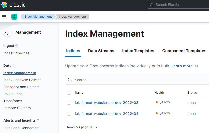
The second system I was looking for was Kibana connected to Elasticsearch. I consider the fact that there are installations on port 80 as an obvious example of a configuration error, because by default Kibana runs on port 5601, so someone had to reconfigure or set up a reverse proxy.
Fig. Opening the available configuration of the Kibana installation
Providing Kibana may result in the display of indexes (logs, metrics and network packages), including the possibility of downloading or even deleting them. By default, the interface does not allow you to retrieve the content of indexes, but if you use the appropriate console tool, it will be able to do so. Often times, if port 80 contains Kibana, the 9200 and 9300 contain Elasticsearch services, also publicly available. As part of the Elasticsearch and Kibana systems, we have one more service, namely the APM server, i.e. application monitoring.
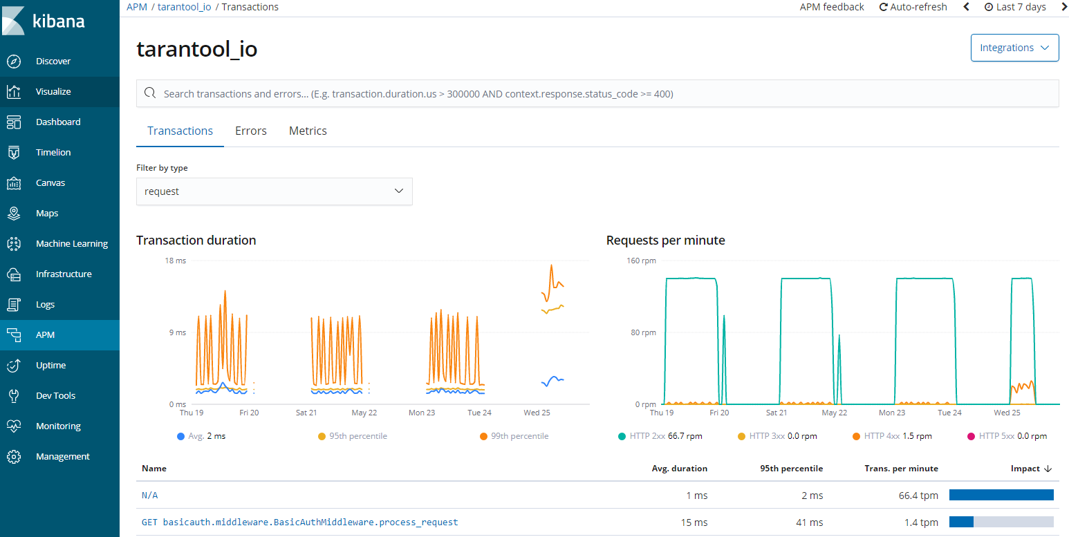
Fig. APM server
Exposing diagnostic data about the application results in increased possibilities of exploring such an application, because APM provides information about the database, related services and addresses on which the application operates on the HTTP layer. Elasticsearch, beats and Kibana is a powerful tool that can give us a lot of information in the form of a reconnaissance of the network environment.
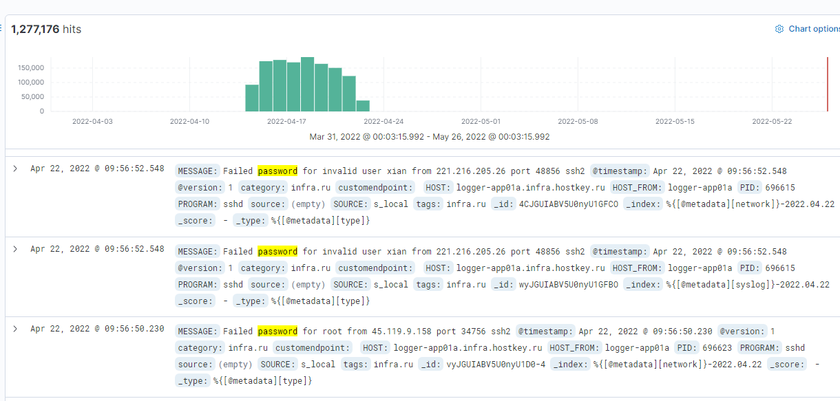
Fig. High exposure of infrastructure details
Files listing
The third type of resource is file stores in the form of file listings on the HTTP server . I found almost 3000 of such installations. Among the more interesting finds I can mention copies of databases, video surveillance archive or code repositories . There are also scans of documents, bank transfer confirmations, certificates and many more. Some users of these servers may not know they have a public IP. Their IP can be dynamic but public. The second category are people who think that only they know this IP address, which is an obvious mistake, because addresses are commonly known.
Note: Domain addresses (especially subdomains) are not widely known, unless we are talking about reverse DNS mapping. The DNS issue is material for the next article.
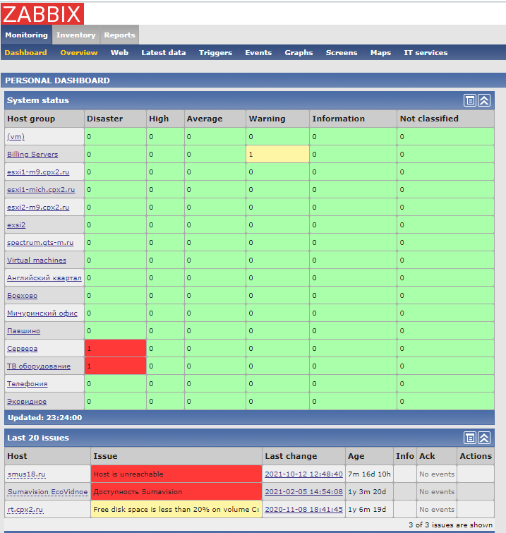
Zabbix
The fourth type is 636 Zabbix monitoring system installations. It should be on a private network with access behind WAF or VPN, but that’s not the case in these cases. Moreover, many of them allow access under the guest account. Basically, it is wrong that such data is publicly available because it identifies the system on multiple layers.
Fig. Access to Zabbix on the guest account
We learn that the systems are run on VMware, what is the logical division of the application, etc. We obtain information about addressing. This can be the basis for further exploration of this particular organization.
Grafana
As in the case of Kibana and Zabbix, the same Grafana, if unsecured, provides us with a lot of valuable information about the system infrastructure, addressing and resource usage. It is a base for further exploration.
Fig. Infrastructure monitoring
The situation is even more interesting because we have the ability to create our own screens, where we can place control panels or multi-level monitoring. This is also the case with the most interesting example that was found in this scan run.It is a monitoring and control panel for heating devices.
Fig. Monitoring and control panel for heating devices
I’ve seen various panels, mainly related to video surveillance, wind turbines or photovoltaics, but I haven’t found such one before. Since someone provides monitoring and buttons to perform various actions (on another panel), I suppose it may have an impact on the operation of physical devices. Therefore, we are entering a dangerous area, because the devices work with high temperature and pressure and it would be bad if they worked outside the parameters. Right?
Note: Some of the systems released to the public are either testing or abandoned systems. Some are clearly honey-pot systems. Most, that is, almost all, however, are production systems or will become production systems in some time. Regardless of their nature, they should not be available to the public, as it is against good practice.
Going to the end
Turkish cryptocurrency exchange
For the ones who managed to make it to the end of this article, there will be one more curiosity. Well, in 2021, when I made my first attempts to scan, in 200 territories I found something more interesting than the finds described here. The scanning did not cover Turkey, but the country where the Turkish cryptocurrency exchange was located. I found a log monitoring system that stored usernames and their passwords. This data allowed access to the accounts . That is why it is so important to inventory resources, check configuration and perform security audits.
Note: The system explorations described are just an example. They do not cover all possible services, or even analyze everything that has been identified. In no way was the obtained information and access used against anyone. Neither of the systems has been tampered with.
Contact
If you are interested in this article, please do not hesitate to contact me. I am open to various forms of cooperation, both commercial and non-commercial, in the field of infrastructure, architecture and security.
A semiconductor is a material whose electrical conductivity is between the conductors and insulators. Their resistance and conductivity depends on temperature and admixtures. [W] The most commercially used semiconductors are those based on silicon, and in the past also on germanium. In addition to these two elements (in crystalline form), a whole spectrum of other substances from groups 13-15 is used, which can form two, three or four-element compounds.
P-n junction
The basic element of a semiconductor system
[003] Additions of atoms of other elements are used to obtain the increased conductivity of the semiconductors. For example, arsenic or antimony causes the appearance of free electrons, which are a source of negative charges. These semiconductors are of the n (negative) type. In turn, indium and barium cause a shortage of electrons, because their atoms take electrons from the environment from silicon atoms, causing the formation of positive charges. They are p (positive) semiconductors. N-type and p-type semiconductors, joined together by a special technological process, form an essential part of each semiconductor element, called the p-n layer. At the boundary of these semiconductors, a p-n junction is formed, carrying current from p to n.
Semiconductor diode
Component of the construction of rectifiers and signaling elements
[003] A two-element component (di or two), intended for example for the construction of rectifiers, protections or, in the case of LEDs, also as a signaling or lighting element. It is a p-n junction with a resistance in the forward direction approx. 10,000 times lower than in the reverse direction.
[101] The diodes can be used to recreate the amplitude of the signal, shift the signal by a constant component or multiply the voltage.
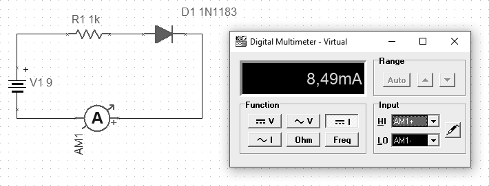
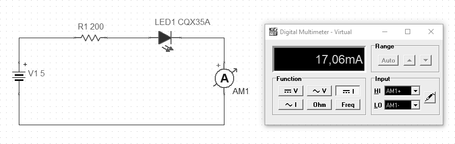
[202] A silicon diode should be connected in the direction of the symbol’s arrow if we want it to conduct current. Setting it in the opposite way is a blockage state in which there should be no conduction up to a certain voltage. If we exceed the parameters of the designed operation of such diodes, then it will be damaged and can conduct current in both directions.
Fig. LED in forward direction (p09)
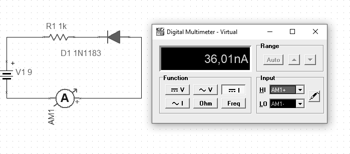
If the diode is connected in the reverse direction, the measured current should be negligible. In the example below, the current is approximately 36 nA.
Fig. LED connected in blocking (p10)
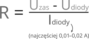
The voltage drop across the diodes (here LED) depends on the substance used, which determines the given color of the luminescence. These drops usually occur from 1.7 to 3.6 V. The diodes have specific operating parameters and when supplying voltage to the system, make sure that the current value is correct, which is limited by a series resistor. The order of connection in the series connection in this case does not matter, so the resistor can be both before and after the diode.
Eq. The required resistance of the resistor to power the diode
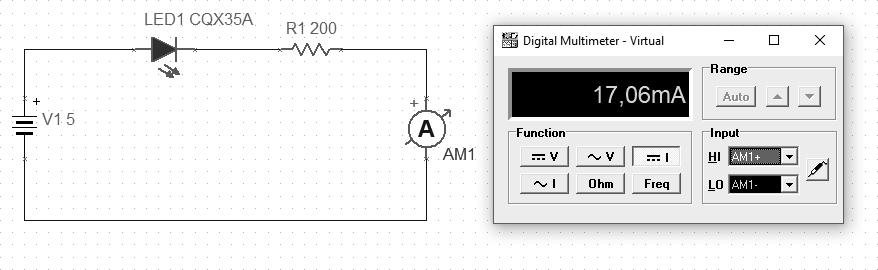
To illustrate that the order of connection of the resistor and diode does not matter, below are two similar examples to illustrate.
Fig. Resistor “before” the diode (p11)
We get the same result in both examples.
Fig. Resistor “after” the diode (p12)
The current can be translated as an analogy of water pressure in a closed system, so the order will not be of particular importance when connecting elements in series.
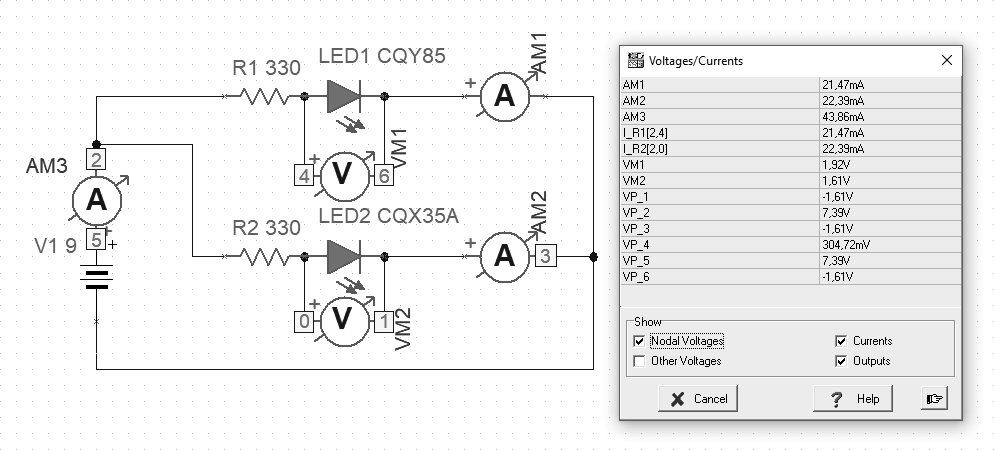
Fig. Parallel connection of series diode + resistor (p13)
The diodes can be connected in series as above. Important operating parameters are forward voltage, standard and maximum current, and reverse parameters. Knowing these parameters, we can choose the appropriate resistors and arrange the whole into a circuit as above.
“The German physicist Ferdinand Braun, a 24-year-old graduate of the University of Berlin, studied the characterization of electrolytes and conductive crystals at the University of Würzburg. In 1874, while examining galena crystals (lead sulfide) with the tip of a thin metal wire, he noticed that the current was flowing freely in only one direction. Braun discovered the electric straightening effect that occurs where metals meet certain crystalline materials. Braun demonstrated this semiconductor device in Leipzig in 1876, but it did not find any useful application until the advent of radio in the early 1900s.” [207]
Zener diode
Reference voltage source
[101] Zener diodes are most often used as an almost constant voltage reference source. If the input voltage is less than the zener voltage, the diode is non-conductive and will not stabilize the voltage.
Fig. The zener diode is connected to the block (p14)
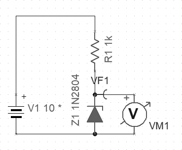
[209] A zener diode is always used as a stabilizer in reverse biased conditions. A Zener diode DC voltage regulator circuit can be designed to provide a constant voltage across the load regardless of changes in input voltage or load current.
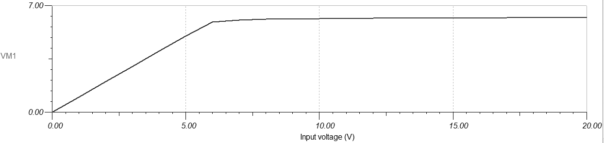
Fig. Measurement of the breakdown voltage
As you can see in the above diagram, the value of the breakdown voltage for the 1N2804 model of the Zener diode is 6.8V, according to the catalog note.
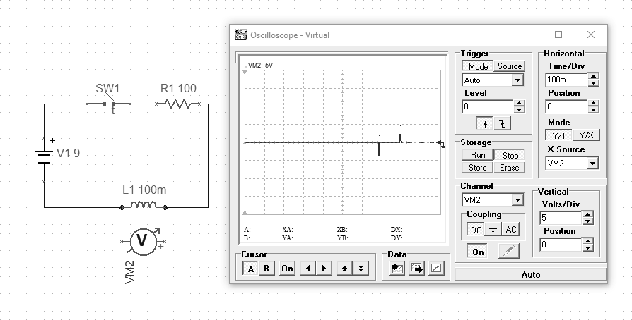
[209] Just as a capacitor works by storing energy as an electric field, an inductor stores energy as a magnetic field. The energy stored in the coil is calculated in terms of current. The capacitor acts as an insulator of the circuit while the inductor acts as its conductor. The coils have inductance expressed in henry [H]. The coils are plugged into the circuit in series with the powered device. The coils are characterized by a maximum current, as their windings have a certain resistance, therefore the flow of current causes a voltage to accumulate on them, which gives the power released by them. Adjusting the operating parameters is to avoid overheating of the coil.
Fig. Difference between continuous power supply and periodic power supply (p08)
The above example (with a cyclic trigger) illustrates the property of the coil of the occurrence of a reverse electromotive force. If we apply voltage constantly, the coil will behave like a piece of wire. However, if there are changes in the intensity of the current flowing through the coil, then we can observe the signal jumps on the measurement.
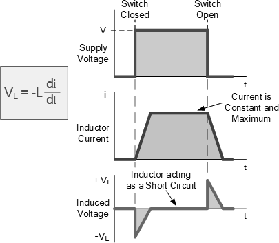
Fig. Voltage and current in a coil [209]
“The use of electric transformers and inductors in the electrical sphere is such a common practice that it is difficult to imagine a world without these devices. When the property of inductance was discovered in the 1830s by Joseph Henry and Michael Faraday (separately and on different continents), the technology was revolutionized. Inductance was first discovered by Faraday in a simple but strange way: he wrapped a paper cylinder in wire, fastened the ends of the wire to a galvanometer (an electric current measuring device), and moved the magnet to and from the cylinder. The galvanometer reacted by revealing that it was producing a tiny current. ” [201]
I will start with the werid experience with one of WP themes – Polite and Polite Grid. I was wondering why my website make double requests on every page. One for the document and other for content. This was annoying as I was unable to measure traffic properly. It turned out that it was because of the theme I’ve been using for some time. Changing it to different one fixed it.
Second of all to make NGINX logs easier to handle I’ve created separate location entry for all the WP things, so the “real” traffic goes only to particular log and everything else goes in different place. Take a look:
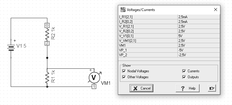
[202] The next example I want to present in practice is a popular voltage divider. It allows the output voltage to be reduced to the desired value due to the properties described a little earlier.
Eq. The output voltage at the divider
Bearing in mind the above formula, we can assume that we want to reduce the input voltage of 5V to the expected 2.5V at the output. So we use two 1K resistors connected in series.
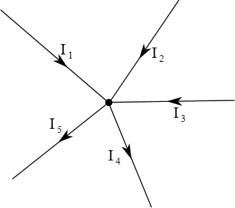
[W] One of the basic principles of current flow is the first law of Kirchhoff, which says that for the electric circuit node, the algebraic sum of flow rates is zero. The sum of currents flowing into the node is equal to the sum of currents flowing out of this node. This law results from the principle of keeping the load.
Fig. Kirchhoff’s first law
Kirchhoff’s second law says that the sum of voltage drops in a closed circuit is zero, assuming that the voltage drop is its negative increase.
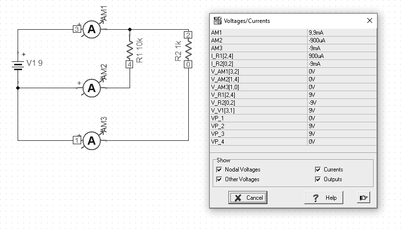
[202] For the purposes of illustrating the law of Kirchhoff, I prepared a simple example below. We start with an example about the first law. 2 resistors are connected, 10k and 1k respectively. We attach 3 ammeters in turn. Sum currents from the circuits of subsequent resistors give the current value for the entire circuit. We can measure this current at a point where there is 1 entrance and 2 outputs.
Fig. Kirchhoff’s first law (P04)
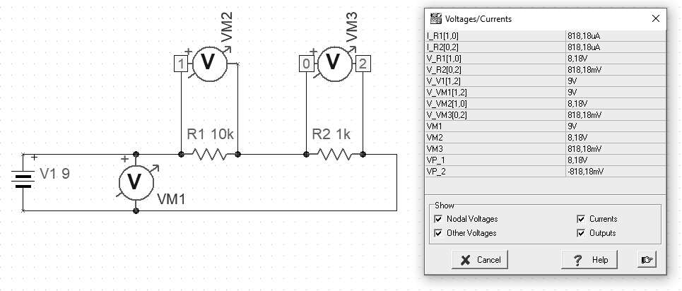
Another example is illustrated by Kirchhoff’s second law. An example shows the difference in the way the circuit elements are connected. By connecting the same voltage values in parallel. By connecting the sum of voltage drops on individual elements, connecting to individual elements.
Fig. Second Law Kirchhoff (P05)
“Gustav Robert Kirchhoff (born March 12, 1824 in Königsberg, died October 17, 1887 in Berlin) – a German physicist, creator of thermal radiation law regarding the relationship between emission and absorption capacity, and rights regarding electrical circuits (first and second law of Kirchhoff)” [W]